一、论文基本信息

报告基本信息

论文标题

FQ-Eval: Building Evaluation Dataset for User-centered Follow-up Question Generation

发表会议

2025 Conference on Empirical Methods in Natural Language Processing (EMNLP 2025) Industry Track

论文地址

https://aclanthology.org/2025.emnlp-industry.188.pdf

开源地址

https://github.com/LGAI-Research/FQ-Eval

二、研究背景与问题提出

2.1 研究背景

随着 ChatGPT、Copilot、Perplexity 等对话式 LLM 服务的规模化落地，后续问题生成（Follow-up Question Generation） 已成为提升用户体验的核心功能：

1. 大量用户难以清晰、完整地向 LLM 表达自身潜在意图与对话目标，模糊查询易导致对话偏离用户初衷，显著降低使用满意度；
2. 高质量的后续问题可降低用户持续交互的门槛，引导用户深化对话、达成核心目标，直接影响商用 LLM 产品的用户留存与活跃度。

2.2 现有研究的核心缺陷

现有后续问题生成相关研究存在三大关键短板，无法适配真实商用 LLM 场景的需求：

1. 评估维度严重片面：绝大多数研究仅聚焦于「信息检索能力」「主题相关性」两个维度，完全忽视了后续问题对用户内在需求的满足、对用户对话目标的支撑，生成的问题与用户真实预期严重脱节；
2. 缺乏标准化评估框架：领域内尚无统一、可复现的用户中心式评估方法，不同研究的评估指标、数据集差异极大，无法横向对比模型性能；
3. 数据集与真实场景脱节：现有主流数据集（如 FQ-Bank、FollowupQG）多基于合成文本、社交平台非正式对话构建，无法反映商用 LLM 服务中用户的真实使用场景与交互模式。

2.3 核心研究问题

如何构建一套贴合真实商用 LLM 使用场景、以用户为中心的后续问题生成评估体系，包括标准化的评估准则、高质量的评估数据集，以及可复现的评估方法，全面衡量后续问题对用户的真实价值。

三、核心研究内容：任务定义与评估准则

3.1 任务形式化定义

论文首次正式定义了商用 LLM 场景下的后续问题生成任务与评估任务，明确了任务边界：

1. 生成任务：给定单轮用户问题 $q \in Q$ 与对应 LLM 回答 $a \in A$ ，通过生成函数 $F$ 输出有价值的后续问题 $f$，即：$f=F(q,a), F:Q \times A \to F$
2. 评估任务：分为两种可互补的范式

• 相对评估（n-way 选择）：给定 QA 对、评估准则与多个候选后续问题，评估函数 $E$ 选出最符合准则的最优问题；
• 绝对评估（分数制）：给定 QA 对、评估准则与单个候选后续问题，评估函数 $E$ 输出 1-5 分的质量评分，分数越高代表与准则的对齐度越好。

3.2 五大用户对齐评估准则（核心创新）

论文通过三阶段用户研究（半结构化访谈→焦点小组讨论→亲和图分析），招募 9 名有丰富 LLM 使用经验、覆盖教育 / 设计 / 编程 / 产品等多元背景的参与者，最终提炼出 5 个完全贴合用户真实预期的评估准则，彻底突破了现有研究仅关注相关性的局限。

四、FQ-Eval 数据集构建

论文构建的 FQ-Eval 是领域内首个基于真实生成式 AI 使用场景、以用户为中心的后续问题生成评估数据集，构建流程全程遵循「真实场景锚定 - 人工精制校准 - 多轮质量管控」原则，确保数据集的可靠性与代表性。

4.1 数据集整体规模

• 核心单元：200 个单轮 QA 对，覆盖 6 大真实生成式 AI 使用类别；
• 标注内容：1000 个人工精制的后续问题，每个 QA 对对应 5 个问题，分别与 5 大评估准则一一对应；
• 对话类型：单轮对话式 QA，适配商用 LLM 的主流交互场景。

4.2 分阶段构建流程

阶段 1：种子 QA 对生成（真实场景锚定）

1. 场景来源：基于哈佛商业评论（HBR）2025 年发布的《生成式 AI 真实使用报告》，覆盖 100 个真实用户生成式 AI 使用场景，分为内容创作、创意娱乐、学习教育、个人 / 职业支持、研究分析、技术支持 6 大类别；
2. 候选生成：为每个场景设计简单、复杂 2 个难度等级，通过 GPT-4.1 为每个难度生成 5 个候选用户问题，总计 1000 个候选种子问题；
3. 人工筛选修订：3 名训练有素的标注员独立评估，从每个难度的 5 个候选中选出 1 个最贴合真实用户语言习惯、场景对齐度最高的问题，最终形成 200 个高质量种子问题；
4. 回答生成与质检：通过 GPT-4.1 为每个种子问题生成对应回答，标注员审核回答的上下文连贯性与完整性，形成最终的 200 个 QA 对。

阶段 2：后续问题筛选与精制（准则对齐）

1. 候选生成：针对每个 QA 对 + 每个评估准则，通过 GPT-4.1 生成 8 个严格贴合准则定义的候选后续问题，每个 QA 对总计生成 40 个候选；
2. 人工筛选与修订：7 名专业标注员（6 名英语母语者 + 1 名双语专家）独立完成两项工作：
   • 筛选：从每个准则的 8 个候选中，选出最能体现该准则核心特征的 1 个问题；
   • 修订：优化选中问题的准则对齐度、上下文连贯性与语言质量，保留核心语义不变；
3. 质量管控：通过 GPT-4.1 对所有最终问题进行自动打分，得分低于 2 分的问题触发人工复检与重标注，确保所有问题与准则的高度对齐。

4.3 与现有主流数据集的对比

五、实验设计与核心结果

论文通过多组互补实验，全面验证了 FQ-Eval 数据集的有效性、评估框架的可靠性，同时揭示了当前主流 LLM 在后续问题生成上的核心短板。

5.1 实验基础设置

1. 评估范式：采用「n-way 选择任务 + 分数制评估任务」双范式，确保评估结果的全面性；
2. 评估器设置：
   • 主力评估器：GPT-4.1（temperature=0.0，贪心解码，确保结果可复现）；
   • 金标准验证：独立人类标注员盲测，与数据集构建阶段的标注员完全隔离，避免偏见；
   • 鲁棒性验证：额外采用 Claude Opus 4、Mistral Large、Gemini 2.5 Flash 作为备选评估器；
3. 对比模型：覆盖 OpenAI、Anthropic、Mistral、Google 四大厂商的 12 款主流 LLM，包含旗舰大模型与中小尺寸模型；
4. 工业场景验证：对商用产品 Perplexity 的后续问题生成能力进行实测评估。

5.2 核心实验结果

实验 1：5-way 选择任务（核心验证实验）

实验设置：对每个 QA 对 + 每个准则，构建 5 候选池（1 个 FQ-Eval 基准问题 + 4 款旗舰 LLM 生成的问题），评估者在盲测环境下选出最符合准则的问题，统计各候选的选择率。

核心结果：

1. FQ-Eval 在 5 个准则上的平均选择率显著高于所有主流 LLM，在创意跳跃维度，LLM-judge 选择率 99.5%、人类选择率 92%，几乎碾压所有对比模型；
2. 在引导入门、LLM 赋能、探索范围三个维度，FQ-Eval 的 LLM-judge 选择率均超过 79%，大幅领先对比模型；
3. 仅在语境相关性维度，Claude Opus 4 等旗舰模型展现出竞争力（人类选择率 28.5%，略高于 FQ-Eval 的 24%），验证了现有 LLM 仅在相关性维度有成熟能力，与论文的核心假设一致。

实验 2：2-way 两两对比任务（全模型覆盖）

实验设置：对每个 QA 对 + 每个准则，构建 2 候选池（1 个 FQ-Eval 基准问题 + 1 款待评估 LLM 生成的问题），评估者二选一，统计 FQ-Eval 的胜率。

核心结果：

1. FQ-Eval 在 12 款 LLM 的全量对比中，平均胜率达 86.4%，在所有准则上均占据绝对优势；
2. 在创意跳跃维度，FQ-Eval 对所有模型的胜率均超过 99%，证明当前主流 LLM 完全无法生成符合用户预期的高创意性后续问题；
3. 同厂商内的中小尺寸模型，在部分准则上的表现优于旗舰大模型，核心原因是中小模型的输出更简洁，更适配简单场景的用户需求；
4. 随着用户问题复杂度提升，FQ-Eval 的胜率略有下降，说明旗舰大模型在高复杂度场景下能更好地发挥能力。

实验 3：分数制绝对评估任务

实验设置：对每个候选后续问题，基于 5 大准则进行 1-5 分的独立绝对评分，分数越高代表质量越好。

核心结果（平均分）：

关键结论：

• FQ-Eval 在所有 5 个准则上的平均分均高于主流旗舰 LLM，总分领先幅度显著；
• 语境相关性维度，FQ-Eval 与 Claude Opus 4 几乎持平，再次验证现有模型在该维度的成熟度；
• 创意跳跃维度，FQ-Eval 平均分是对比模型的 2 倍以上，差距极为显著。

实验 4：真实商用服务评估

核心发现：Perplexity 的后续问题仅在信息检索相关的探索范围、语境相关性维度表现尚可，但在LLM 赋能、引导入门、创意跳跃三个维度表现极差，与 FQ-Eval 的基准水平差距显著。证明 FQ-Eval 可直接用于商用产品的能力诊断，帮助开发者定位优化方向，平衡产品的质量、成本与延迟。

5.3 鲁棒性验证

1. LLM-judge 一致性：4 款不同厂商的 LLM 作为评估器时，两两之间的皮尔逊相关系数均 > 0.8（p<0.001），整体评分相邻一致性（分差≤1 分）达 97.2%，证明评估结果稳定可靠，无系统性偏差；
2. 人类与 LLM-judge 对齐性：人类标注结果与 GPT-4.1 的评估结果高度一致，无显著差异，证明 LLM-judge 的自动化评估完全贴合人类真实偏好；
3. 循环性偏见规避：针对 “GPT-4.1 同时参与数据集构建与评估” 的潜在偏见，论文通过人工修订消除模型风格偏差、人类评估对齐、多模型交叉验证三种方式，证明结果无循环性偏见。

DAPO 简介

在大模型强化学习（RL）训练领域，OpenAI 的 O1、DeepSeek 的 R1 等模型凭借出色的复杂任务表现，证明了大规模 RL 训练的巨大价值。但这些顶尖模型的核心训练技术细节长期未公开，而主流的 GRPO 算法在长链式思维（CoT）等复杂场景中，又频繁面临熵崩溃、训练不稳定等问题。

DAPO（Decoupled Clip and Dynamic Sampling Policy Optimization） 算法针对这些问题，提出了四项关键改进，在保持训练稳定性的同时显著提升了模型在复杂推理任务上的表现。本文将深入剖析 DAPO 的技术原理，重点解析其核心改进点及实际应用价值。

DAPO 的技术背景与核心定位

传统 RL 训练的痛点

GRPO 作为大模型 RL 训练的主流算法，虽能提升模型性能，但在数学推理等长 CoT 场景中暴露出诸多缺陷：

1. 熵崩溃：固定剪裁范围限制了低概率 token 的探索，导致策略快速收敛，生成内容同质化严重
2. 梯度失效：训练后期易出现大量全优或全差样本，优势函数趋近于零，梯度信号消失，浪费训练资源
3. 梯度稀释：长序列样本的梯度经样本级平均后被弱化，关键推理步骤的优化信号无法有效传递
4. 奖励噪声：对超长响应的刚性截断惩罚，易误判有效推理内容，干扰模型对奖励信号的学习

DAPO 的核心目标

DAPO 以”解决长序列 RL 优化难题、提供开源可复现方案、突破复杂任务性能上限”为核心目标。其算法设计围绕”释放模型探索能力、提升训练信号质量、精准优化长序列”三大方向展开，在 AIME 等数学推理任务中取得了显著的性能提升。

DAPO 的四大核心改进点深度解析

DAPO 通过解耦剪辑策略、动态采样机制、token 级损失计算和长度感知奖励修正四项革新，针对性解决了 GRPO 的核心痛点。以下结合技术原理、解决路径和实际效果展开说明：

改进一：Clip-Higher——解耦高低剪辑范围，平衡探索与利用

传统算法的局限

GRPO 和 PPO 均采用固定的对称剪辑范围（如 $\epsilon=0.2$），将新策略与旧策略的概率比值限制在 $[1-\epsilon, 1+\epsilon]$ 区间。传统的剪辑函数为：

其中 $rt = \frac{\pi\theta(at|s_t)}{\pi{\theta_{old}}(a_t|s_t)}$ 是重要性采样比率。

这种设计虽能避免策略突变，但会严重抑制低概率关键 token 的优化。当模型偶然生成一个对推理至关重要但概率极低的 token 时，其概率比值极易超出剪辑上限而被截断，导致该 token 无法获得有效强化，最终模型探索能力衰退，陷入熵崩溃。

DAPO 的解决方案

DAPO 提出解耦式剪辑策略，将上下剪辑阈值拆分为独立参数：

其中：

• 低阈值 $\epsilon_{low}=0.2$：保持与传统算法一致，抑制高概率 token 的过度利用，避免模型陷入局部最优
• 高阈值 $\epsilon_{high}=0.28$：放宽对高比值的限制，为低概率关键 token 提供足够的上涨空间

这种非对称设计既保证了训练稳定性，又释放了模型的探索潜力。例如在数学推理中，模型生成的”辅助变量假设”等低概率关键推理步骤，能通过该机制获得有效强化，逐步形成更完整的推理链条。

实际效果

该改进使模型生成多样性显著提升，训练过程中熵值保持稳定。通过允许更大的上行剪辑范围，模型能够更好地学习低概率但高价值的 token，有效缓解了熵崩溃问题。

改进二：Dynamic Sampling——动态过滤无效样本，强化梯度信号

传统采样的核心问题

训练过程中，当模型性能提升到一定阶段，易出现大量全正确或全错误的样本。这些样本的优势函数值为零，对应的梯度信号也会消失，导致”采样量大但有效信息少”的资源浪费。

在强化学习中，优势函数定义为：

当奖励为极端值（0 或 1）时，$A(s_t, a_t) \approx 0$，导致策略梯度：

趋近于零，训练效率严重下降。

DAPO 的动态采样策略

DAPO 引入梯度有效性筛选机制，具体算法如下：

1
2
3
4
5
6
7
8
9
10
11
12
13
14
15
16
17
18

def dynamic_sampling(model, prompts, target_batch_size):
    effective_samples = []
    sampling_attempts = 0
    
    while len(effective_samples) < target_batch_size:
        # 生成候选样本
        candidates = sample_responses(model, prompts)
        
        # 筛选有效样本（奖励不为极端值）
        for sample in candidates:
            if 0 < sample.reward < 1:  # 排除极端奖励
                effective_samples.append(sample)
                
        sampling_attempts += 1
        if sampling_attempts > max_attempts:
            break
    
    return effective_samples[:target_batch_size]

该机制的核心逻辑是：若当前采样结果中无有效梯度样本，则触发二次采样，直至批次中充满具备梯度价值的样本。由于过滤操作仅需校验奖励值，计算开销极低，不会显著增加训练时间。

实际效果

动态采样使模型收敛速度大幅提升，通过确保每个训练批次都包含有效的梯度信号，避免了训练后期因梯度失效导致的模型性能震荡。实验表明，该机制能够显著提升训练效率。

改进三：Token-Level Policy Gradient Loss——精准优化长序列，避免梯度稀释

长序列优化的核心痛点

GRPO 采用”样本内平均+批次内平均”的双层损失计算方式。传统的损失函数为：

其中 $B$ 是批次大小，$T_i$ 是第 $i$ 个样本的序列长度，$\ell_t^{(i)}$ 是第 $i$ 个样本第 $t$ 个 token 的损失。

这种方式对长序列极不友好：一个 200 token 的长回答与一个 10 token 的短回答，在样本级平均后，每个 token 的梯度权重分别为 $1/200$ 和 $1/10$。长回答中的关键推理 token（如公式推导、逻辑转折）的梯度被严重稀释，模型难以捕捉长链式推理的核心规律。

DAPO 的 token 级损失计算

DAPO 将损失聚合方式从样本级改为全局 token 级：

其中 $w_t^{(i)}$ 是第 $i$ 个样本第 $t$ 个 token 的权重。

具体优化包括：

1. 取消样本内梯度平均：直接计算每个 token 的独立损失
2. 全局归一化：按批次内所有 token 的总数进行归一化，而非按样本数量归一化
3. 重要性权重：对长序列中的关键 token（如数学公式、逻辑连词）可额外增加权重

1
2
3
4
5
6
7
8
9
10
11
12

def token_level_loss(batch_outputs, advantages):
    total_tokens = sum(len(output) for output in batch_outputs)
    token_losses = []
    
    for output, advantage in zip(batch_outputs, advantages):
        for token_id, token_advantage in zip(output, advantage):
            # 每个token独立计算损失，无样本内平均
            token_loss = -log_prob(token_id) * token_advantage
            token_losses.append(token_loss)
    
    # 全局token级归一化
    return sum(token_losses) / total_tokens

这确保长、短回答的每个 token 拥有公平的梯度权重，长序列中的有效信息不再被稀释。

实际效果

该改进让模型的长序列生成能力显著增强。在需要多步骤推理的数学题求解中，模型能稳定生成结构完整的推理过程，重复、乱码等低质量模式大幅减少，训练稳定性也得到明显提升。

改进四：Overlong Reward Shaping——软惩罚机制，降低奖励噪声

传统长度惩罚的缺陷

传统算法对超长响应采用刚性惩罚（如超过长度阈值直接扣 1 分），这种方式存在两大问题：

1. 误判有效内容：将有效长推理与无效冗余内容同等惩罚，例如完整的数学推导因超长被误判为低质量
2. 引入奖励噪声：突然的惩罚会引入剧烈奖励噪声，干扰模型对有效推理模式的学习

DAPO 的长度感知奖励修正

DAPO 设计了分段式软惩罚函数，根据响应长度动态调整惩罚力度：

其中 $l{\text{max}}$ 为最大长度阈值，$l{\text{cache}}$ 为缓冲长度。该函数实现三层惩罚逻辑：

1. 正常长度区间：无惩罚，鼓励完整推理
2. 缓冲区间：惩罚随长度线性增加，避免轻微超长被过度惩罚
3. 超长区间：刚性惩罚，过滤无意义的冗余内容

最终的奖励函数为：

其中 $\alpha$ 是长度惩罚的权重系数。

同时，DAPO 会过滤截断样本的损失计算，进一步减少噪声对训练的干扰：

1
2
3
4
5
6
7

def compute_length_penalty(response_length, max_length=2048, cache_length=512):
    if response_length <= max_length - cache_length:
        return 0.0
    elif response_length <= max_length:
        return (max_length - cache_length - response_length) / cache_length
    else:
        return -1.0

实际效果

软惩罚机制使训练波动大幅降低，模型既能生成足够长度的推理内容，又能有效抑制无意义的冗余输出，实现了推理完整性与简洁性的平衡。

DAPO 的整体训练流程与性能表现

完整训练流程

DAPO 的训练流程整合了四项核心改进，具体步骤如下：

1. 数据预处理：输入 prompt 与高奖励回复数据，标注 token 级别重要性与响应长度信息
2. 动态采样：过滤无效样本，构建梯度有效的训练批次
3. 策略优化：基于 Clip-Higher 计算策略比值，通过 token 级损失函数反向传播梯度
4. 奖励修正：采用软惩罚函数调整超长响应的奖励值，更新模型参数
5. 迭代优化：循环上述步骤，直至模型熵值稳定且任务准确率达到目标

算法伪代码

1
2
3
4
5
6
7
8
9
10
11
12
13
14
15
16
17
18
19
20
21
22
23
24
25
26
27
28

def dapo_training(model, dataset, epochs):
    for epoch in range(epochs):
        # 1. 动态采样
        effective_batch = dynamic_sampling(model, dataset.prompts)
        
        # 2. 计算重要性采样比率 (Clip-Higher)
        ratios = []
        for sample in effective_batch:
            old_prob = old_model.log_prob(sample)
            new_prob = model.log_prob(sample)
            ratio = exp(new_prob - old_prob)
            clipped_ratio = clip_higher(ratio, eps_low=0.2, eps_high=0.28)
            ratios.append(clipped_ratio)
        
        # 3. Token级损失计算
        loss = compute_token_level_loss(effective_batch, ratios)
        
        # 4. 长度感知奖励修正
        adjusted_rewards = []
        for sample in effective_batch:
            length_penalty = compute_length_penalty(len(sample))
            adjusted_reward = sample.reward + length_penalty
            adjusted_rewards.append(adjusted_reward)
        
        # 5. 反向传播更新
        optimizer.zero_grad()
        loss.backward()
        optimizer.step()

性能表现分析

实验结果显示 DAPO 在数学推理任务上的显著提升：

从数据可见，DAPO 的四项改进形成了协同效应，每项改进都对最终性能有积极贡献。特别值得注意的是，训练过程中模型还自发演化出”反思修正”等高级推理能力，证明其优化方向贴合复杂任务的核心需求。

总结与展望

核心贡献

DAPO 的核心价值体现在以下几个方面：

1. 系统性解决方案：针对 GRPO 在长序列训练中的四大痛点，提出了对应的解决方案
2. 技术创新：解耦剪辑策略和 token 级损失计算等创新设计，为强化学习优化提供了新思路
3. 实用性：显著的性能提升证明了算法的实际价值，特别是在数学推理等复杂任务上

技术优势总结

未来发展方向

DAPO 的优化方向可能集中在以下几个方面：

1. 自适应参数调整：根据训练阶段和任务特性，动态调整 Clip-Higher 的阈值参数
2. 智能权重分配：结合注意力机制，为不同类型的 token 分配更精准的权重
3. 多任务适配：扩展到更多领域的复杂推理任务，验证算法的通用性
4. 计算优化：进一步优化动态采样的计算效率，降低训练开销

实际应用价值

对于研究人员而言，DAPO 提供了一套完整的长序列强化学习优化框架，为探索更高效的大模型训练路径提供了重要参考。对于工业界来说，其高效的训练策略为降低大规模模型的训练成本、提升复杂任务性能提供了实用的解决方案。

通过解决长序列强化学习的核心技术难题，DAPO 为大模型在复杂推理任务上的应用奠定了更加坚实的基础。

在 GRPO 博文中，我们详细介绍了 GRPO 的 token 级优化方法。本文深入探讨 GSPO 的算法原理，以及与 GRPO 的核心区别。

GSPO 的核心创新：

1. 序列级重要性采样：不计算每个 token 的重要性比率，而是计算整个序列的重要性比率
2. 几何平均归一化：通过开方操作消除序列长度对概率乘积的影响
3. 好坏序列对比学习：直接通过好序列和坏序列的对比来计算优势
4. 更稳定的训练：避免 token 级别方差大的问题

GRPO vs GSPO：概念回顾

GRPO 的 Token 级优化

GRPO（Group Relative Policy Optimization）采用 token 级别 的优化策略：

核心特点：

1. Token 级重要性采样：对每个 token 计算 $rt^{\text{(i)}} = \frac{\pi\theta(at^{(i)}|s_t^{(i)})}{\pi{\text{ref}}(a_t^{(i)}|s_t^{(i)})}$
2. 奖励分解分配：将序列奖励 $r_{\text{RM}}$ 分配到每个 token（通常采用折扣分配）
3. Token 级优势：每个 token 有独立的优势值 $\hat{A}_t^{(i)}$
4. Token 级裁剪：对每个 token 的重要性比率进行 PPO 风格裁剪
5. 损失聚合：先对单序列内的 token 平均，再对 batch 平均

优点：

• 贴合模型逐 token 生成的过程
• 提供精细的梯度信号
• 理论基础清晰（PPO 风格）

缺点：

• Token 级方差大，特别是在长序列中
• 奖励分摊到单个 token 可能出现矛盾
• MoE 模型中某些专家可能退化（处理少数低质量 token）

GSPO 的序列级优化

GSPO（Group Sequence Policy Optimization）采用 序列级别 的优化策略：

核心特点：

1. 序列级重要性采样：计算整个序列的重要性比率 $s(y) = \left(\frac{\pi\theta(y|x)}{\pi{\text{ref}}(y|x)}\right)^{1/L}$
2. 不分摊奖励：直接使用完整序列的整体奖励
3. 几何平均归一化：用 $1/L$ 次方消除序列长度差异
4. 好坏序列对比：通过比较好序列和坏序列的平均重要性比率计算优势
5. 损失聚合：直接对序列计算损失，然后平均

优点：

• 优化目标与人类评价逻辑一致（关注整体质量）
• 序列级方差小，训练更稳定
• 支持长文本和 MoE 模型更好
• 避免分摊奖励的矛盾

缺点：

• 失去 token 级的精细控制
• 无法区分序列内各 token 的贡献
• 不同长度序列的比较可能仍存在偏差

GSPO 的算法原理

1. 序列级重要性采样比率

GSPO 的核心创新是 序列级重要性采样比率，这解决了序列长度不同导致概率乘积差异大的问题。

序列概率计算

对于长度为 $L$ 的序列 $y = (y_1, y_2, \ldots, y_L)$，整个序列的生成概率是所有 token 条件概率的乘积：

类似地，参考模型的序列概率为：

几何平均归一化

简单的概率比 $\frac{\pi\theta(y|x)}{\pi{\text{ref}}(y|x)}$ 存在一个问题：长序列的概率乘积会更小，导致长序列的重要性比率被低估。

例如：

• 短序列（长度 3）：$0.5 \times 0.5 \times 0.5 = 0.125$
• 长序列（长度 10）：$0.5^{10} \approx 0.001$

即使两个序列的 token 概率分布相同，长序列的重要性比率也会被人为降低。

GSPO 的解决方案：使用 几何平均（geometric mean），即开 $L$ 次方：

直观理解：

• 这相当于计算 “平均每个 token 的概率增长倍数”
• 长序列和短序列可以公平比较
• 与序列长度无关

数值例子：

假设一个长度为 $L$ 的序列中，每个 token 的概率都从 0.3 增加到 0.4：

不同长度下的比率：

• $L=3$：$(1.333)^3 \approx 2.37 \rightarrow$ 开 3 次方 $= 1.333$
• $L=10$：$(1.333)^{10} \approx 33.9 \rightarrow$ 开 10 次方 $= 1.333$

经过几何平均，得到相同的 $s(y) = 1.333$，公平地反映了两个序列的改进程度。

对数概率视角

为了数值稳定性，实践中通常用对数形式：

或者：

这样避免了浮点数下溢。

2. 组内优势计算

与 GRPO 不同，GSPO 不计算单个序列的绝对优势，而是计算 组内相对优势——即好序列相对于坏序列的优势。

序列分组

对于一个 batch 中的 $B$ 个 prompt，每个 prompt 采样 $G$ 个序列，得到 $B \times G$ 个序列。

对于每个 prompt，按奖励将 $G$ 个序列分成两组：

• 好序列组 $G_{\text{good}}$：奖励高于组内平均的序列
• 坏序列组 $G_{\text{bad}}$：奖励低于组内平均的序列

分组标准：

• 若 $r_i > \bar{r}$：序列 $i$ 属于好序列组
• 若 $r_i < \bar{r}$：序列 $i$ 属于坏序列组

组内平均重要性比率

计算两组的平均重要性比率：

序列级优势

序列级优势定义为两组平均重要性比率的差：

含义：

• 若 $A > 0$：新策略目前更倾向生成好序列（方向正确）
• 若 $A < 0$：新策略目前更倾向生成坏序列（需要调整）

注意：这里的优势是 全局的，所有好序列和坏序列之间的平均比较。

3. 损失函数

GSPO 的损失函数包含两部分：策略损失和 KL 约束。

策略损失

或使用 PPO 风格的裁剪：

其中 $\epsilon = 0.2$ 是裁剪范围。

目标：

• 提高好序列的整体生成概率（$\bar{s}_{\text{good}}$ 增大）
• 降低坏序列的整体生成概率（$\bar{s}_{\text{bad}}$ 减小）
• 限制更新幅度（通过裁剪）

KL 约束

这里对整个序列计算 KL 散度，防止策略偏离参考模型太远。

总损失

其中 $\beta$ 是 KL 权重（通常 0.01-0.1）。

GSPO vs GRPO 的详细对比

重要性采样粒度对比

优势计算对比

梯度更新对比

性能对比

GSPO 的实现细节

1. 序列级重要性比率计算

伪代码

1
2
3
4
5
6
7
8
9
10
11
12
13
14
15
16
17
18
19
20
21
22
23
24
25
26
27
28
29
30
31
32
33
34
35
36
37
38
39
40

def compute_sequence_importance_ratio(actor_logits, ref_logits, 
                                     token_ids, sequence_lengths):
    """
    计算序列级重要性比率
    
    Args:
        actor_logits: shape (B, G, T, V) - Actor 模型 logits
        ref_logits: shape (B, G, T, V) - Reference 模型 logits
        token_ids: shape (B, G, T) - 生成的 token IDs
        sequence_lengths: shape (B, G) - 每个序列的实际长度
    
    Returns:
        seq_ratios: shape (B, G) - 序列级重要性比率
    """
    B, G, T, V = actor_logits.shape
    
    # 计算 log 概率
    actor_log_probs = log_softmax(actor_logits, dim=-1)  # shape (B, G, T, V)
    ref_log_probs = log_softmax(ref_logits, dim=-1)
    
    # 提取生成 token 的 log 概率
    actor_seq_log_prob = torch.zeros(B, G)
    ref_seq_log_prob = torch.zeros(B, G)
    
    for b in range(B):
        for g in range(G):
            L = sequence_lengths[b, g]
            # 求和所有 token 的 log 概率
            for t in range(L):
                token_id = token_ids[b, g, t]
                actor_seq_log_prob[b, g] += actor_log_probs[b, g, t, token_id]
                ref_seq_log_prob[b, g] += ref_log_probs[b, g, t, token_id]
    
    # 计算序列级重要性比率（取幂化为线性）
    log_ratio = actor_seq_log_prob - ref_seq_log_prob
    
    # 几何平均：除以序列长度
    seq_ratios = torch.exp(log_ratio / sequence_lengths)
    
    return seq_ratios

2. 好坏序列分组与优势计算

伪代码

1
2
3
4
5
6
7
8
9
10
11
12
13
14
15
16
17
18
19
20
21
22
23
24
25
26
27
28
29
30
31
32
33
34
35
36
37
38
39
40
41
42
43
44
45
46
47
48
49
50
51
52

def compute_sequence_advantage(seq_ratios, rewards, sequence_lengths):
    """
    计算序列级优势
    
    Args:
        seq_ratios: shape (B, G) - 序列级重要性比率
        rewards: shape (B, G) - 每个序列的奖励
        sequence_lengths: shape (B, G) - 序列长度
    
    Returns:
        advantages: shape (B, G) - 序列级优势
        group_advantages: shape (B,) - 每个 prompt 的组优势
    """
    B, G = seq_ratios.shape
    
    advantages = torch.zeros(B, G)
    group_advantages = torch.zeros(B)
    
    for b in range(B):
        # 计算该 prompt 的平均奖励
        mean_reward = rewards[b].mean()
        
        # 分组
        good_mask = rewards[b] >= mean_reward
        bad_mask = ~good_mask
        
        good_ratios = seq_ratios[b, good_mask]
        bad_ratios = seq_ratios[b, bad_mask]
        
        # 计算好坏序列的平均重要性比率
        if len(good_ratios) > 0:
            mean_good_ratio = good_ratios.mean()
        else:
            mean_good_ratio = 0.0
        
        if len(bad_ratios) > 0:
            mean_bad_ratio = bad_ratios.mean()
        else:
            mean_bad_ratio = 0.0
        
        # 组优势
        group_adv = mean_good_ratio - mean_bad_ratio
        group_advantages[b] = group_adv
        
        # 每个序列的优势（同组内所有序列相同）
        for g in range(G):
            if good_mask[g]:
                advantages[b, g] = group_adv
            else:
                advantages[b, g] = -group_adv  # 坏序列的优势为负
    
    return advantages, group_advantages

3. 损失计算

伪代码

1
2
3
4
5
6
7
8
9
10
11
12
13
14
15
16
17
18
19
20
21
22
23
24
25
26
27
28
29
30
31
32
33
34
35
36
37
38
39
40
41
42
43
44
45
46
47
48
49
50
51

def compute_loss(actor_logits, ref_logits, token_ids, 
                seq_ratios, advantages, sequence_lengths,
                beta=0.05, epsilon=0.2):
    """
    计算 GSPO 损失
    
    Args:
        actor_logits: shape (B, G, T, V)
        ref_logits: shape (B, G, T, V)
        token_ids: shape (B, G, T)
        seq_ratios: shape (B, G) - 序列级重要性比率
        advantages: shape (B, G) - 序列级优势
        sequence_lengths: shape (B, G)
        beta: KL 权重
        epsilon: 裁剪范围
    
    Returns:
        total_loss: 标量损失
    """
    B, G, T, V = actor_logits.shape
    
    # 计算 log 概率
    actor_log_probs = log_softmax(actor_logits, dim=-1)
    ref_log_probs = log_softmax(ref_logits, dim=-1)
    
    policy_loss = 0.0
    kl_loss = 0.0
    
    for b in range(B):
        for g in range(G):
            L = sequence_lengths[b, g]
            adv = advantages[b, g]
            ratio = seq_ratios[b, g]
            
            # PPO 风格的裁剪
            clipped_ratio = clamp(ratio, 1 - epsilon, 1 + epsilon)
            policy_term = min(ratio * adv, clipped_ratio * adv)
            policy_loss += -policy_term  # 最大化优势，所以取负
            
            # KL 散度（序列级）
            kl_sum = 0.0
            for t in range(L):
                token_id = token_ids[b, g, t]
                log_ratio_t = (actor_log_probs[b, g, t, token_id] - 
                              ref_log_probs[b, g, t, token_id])
                kl_sum += log_ratio_t
            
            kl_loss += kl_sum / L  # 每个 token 的平均 KL
    
    total_loss = (policy_loss + beta * kl_loss) / (B * G)
    return total_loss

4. 超参数设置

调优建议

1. 组大小 $G$：

   • GSPO 对 $G$ 的敏感度低于 GRPO（因为序列级优势更稳定）
   • 推荐从 $G=8$ 开始
   • 如果仍有波动，增加到 $G=16$ 或 $G=32$

2. KL 权重 $\beta$：

   • 观察 KL 散度大小：
     • KL > 0.1：增大 $\beta$
     • KL < 0.01：减小 $\beta$
     • 目标：0.01-0.05
   • GSPO 通常需要更小的 $\beta$（因为更稳定）

3. 学习率：

   • GSPO 对学习率不如 GRPO 敏感
   • 可以用略大的学习率（5e-7）
   • 监测梯度范数，避免梯度爆炸

GSPO 完整数值示例

假设条件

• 批大小：$B = 1$（1 个 prompt）
• 组大小：$G = 3$（3 个序列）
• 序列长度：$L_1 = 5, L_2 = 7, L_3 = 6$（长度不同）
• 奖励：$r_1 = 8, r_2 = 6, r_3 = 4$
• 平均奖励：$\bar{r} = 6$

计算过程

步骤 1: 分组

1
2
3
4
5
6
7
8
9
10

平均奖励: r_bar = (8 + 6 + 4) / 3 = 6

好序列组（r_i >= 6）：
  - 序列 1: r_1 = 8 ✓
  - 序列 2: r_2 = 6 ✓
  
坏序列组（r_i < 6）：
  - 序列 3: r_3 = 4 ✓

分组结果：G_good = {seq1, seq2}, G_bad = {seq3}

步骤 2: 计算序列级重要性比率

假设：

• 序列 1（长度 5）：每个 token 概率比平均 1.1 倍

  • $\log \pi\theta = -0.5$，$\log \pi{\text{ref}} = -0.55$
  • 序列 log 比：$5 \times 0.05 = 0.25$
  • 几何平均：$\log s(y_1) = 0.25 / 5 = 0.05 \Rightarrow s(y_1) \approx 1.051$

• 序列 2（长度 7）：每个 token 概率比平均 1.05 倍

  • 序列 log 比：$7 \times 0.0488 = 0.342$
  • 几何平均：$\log s(y_2) = 0.342 / 7 = 0.049 \Rightarrow s(y_2) \approx 1.050$

• 序列 3（长度 6）：每个 token 概率比平均 0.95 倍

  • 序列 log 比：$6 \times (-0.0513) = -0.308$
  • 几何平均：$\log s(y_3) = -0.308 / 6 = -0.0513 \Rightarrow s(y_3) \approx 0.950$

关键观察：尽管序列长度不同（5, 7, 6），经过几何平均后，序列 1 和 2 的 $s$ 值相近（都约 1.05），反映了相同的改进程度。

步骤 3: 计算组平均重要性比率

1
2
3
4
5
6
7
8

好序列组平均：
  s_good = (s(y_1) + s(y_2)) / 2 = (1.051 + 1.050) / 2 ≈ 1.0505

坏序列组平均：
  s_bad = s(y_3) = 0.950

组优势：
  A = s_good - s_bad = 1.0505 - 0.950 = 0.1005

解释：好序列组的重要性比率高于坏序列组，说明新策略目前倾向于生成好序列，优化方向正确。

步骤 4: 计算损失

假设 $\epsilon = 0.2$，$\beta = 0.05$：

1
2
3
4
5
6
7
8
9
10
11
12
13
14
15
16
17
18
19
20
21
22
23

裁剪重要性比率（假设所有 s 值都在 0.8-1.2 范围内）：
  clipped_good ≈ 1.0505（无需裁剪）
  clipped_bad ≈ 0.950（无需裁剪）

策略损失（对好坏序列分别计算）：
  - 好序列 1: loss_1 = -min(s(y_1) * A, clip(s) * A)
                       = -min(1.051 * 0.1005, 1.051 * 0.1005)
                       = -0.1057
  
  - 好序列 2: loss_2 = -min(1.050 * 0.1005, 1.050 * 0.1005)
                       = -0.1055
  
  - 坏序列 3: loss_3 = -min(0.950 * (-0.1005), 0.950 * (-0.1005))
                       = 0.0955

平均策略损失：
  L_policy = (0.1057 + 0.1055 + 0.0955) / 3 ≈ 0.1022

KL 散度（简化，假设每个 token 的 log ratio 平均 0.05）：
  L_KL ≈ 0.05

总损失：
  L_total = L_policy + β * L_KL = 0.1022 + 0.05 * 0.05 = 0.1047

关键观察：

• 好序列的损失为正（鼓励），坏序列的损失为负（惩罚）
• 通过最小化总损失，模型会学习生成更多好序列
• KL 项保证了模型不会偏离参考模型太远

GRPO vs GSPO 的选择

什么情况下使用 GRPO

1. 短文本任务：生成文本长度一致，token 级方差不大
2. 需要精细控制：想要针对不同位置的 token 进行不同的优化
3. 实验早期：GRPO 理论更清晰，调试更容易

什么情况下使用 GSPO

1. 长文本任务：生成长序列或文本长度差异大
2. 模型规模大：大模型中 token 级波动更明显
3. MoE 架构：避免专家利用率不均衡
4. 追求稳定性：GSPO 训练更稳定，收敛更快
5. 生产环境：GSPO 的鲁棒性更好

实践建议

从 GRPO 迁移到 GSPO 的步骤：

1. 验证 GRPO 的基线：确保 GRPO 训练稳定
2. 调整参数：
   • 保持 $\beta$ 不变（或略减小）
   • 可能需要增加 $G$（因为序列级优势更稳定）
3. 逐步替换：先在部分数据上尝试 GSPO
4. 监控关键指标：
   • KL 散度（应保持在 0.01-0.1）
   • 奖励均值和方差
   • 序列长度分布

总结

GSPO 相比 GRPO 的核心改进：

1. 序列级优化：从 token 级提升到序列级，减少方差
2. 几何平均归一化：公平处理不同长度的序列
3. 好坏对比学习：优化目标更直观、更稳定
4. 更强的鲁棒性：特别是在长文本和 MoE 模型上

关键理解：

• GRPO 和 GSPO 都不需要 Critic 模型
• 两者都使用组内比较来计算优势
• GSPO 的创新在于 将粒度从 token 级提升到序列级

性能对比：

• 训练稳定性：GSPO > GRPO（特别是长文本）
• 收敛速度：GSPO ≥ GRPO
• 计算复杂度：两者相近（GSPO 略高）
• 理论完备性：GRPO（基于 PPO）vs GSPO（创新设计）

推荐阅读：

• GRPO 博文，理解基础概念
• PPO 博文，理解策略梯度方法
• 对比两种算法的优缺点，根据实际场景选择

为什么需要结构化输出？

在实际应用中，我们经常需要 LLM 的输出能够被程序直接解析和使用，而不是仅仅作为文本供人类阅读。结构化的 JSON 输出具有以下优势：

• 可解析性：程序可以直接解析和处理 JSON 数据
• 类型安全：明确的字段类型和结构规范
• 可验证性：可以通过 Schema 验证数据完整性
• 易集成：与现有系统和 API 无缝集成

方法一：提示词 + JSON format

这是最常用的让模型输出 JSON 格式的方法了。首先就是 prompt 中声明要输出 JSON，配合一些样例 few shot，然后呢，类似 Azure、Gemini 这类的大模型调用接口，都有类似 response_format 可以指定输出 JSON 格式。

模式如下：
JSON 提示词描述 + JSON 样例（Few shot）+ JSON response_format 来约束大模型的 JSON 输出。

如何用比较好地用提示词描述 JSON 字段呢？网络上比较好的实践是用 Typescript 或者 Yaml 格式描述（LLM生成Json结构化数据的几种方案，个人目前认为最好的方式依然是`TypeScript约束Prompt + Yaml格），当然简单地就直接用列表描述就好。可以参考这篇文章：https://juejin.cn/post/7325429835387404307

需要注意的点：

• 1. 这个方法不能百分百保证。笔者在 gemini 2.5 pro，指定了 response_format 为 JSON，prompt 给了 few shot，在大型的 JSON 生成的时候，一样会失败。但是 gemini 2.5 pro 指定 json schema，生成成功率大幅度提高。
• 1. 对于没有 json schema 参数的接口，few show 中的 json 样例非常重要。

再说一下这些 API 提供的 JSON response format，本质是一个 Constrained Decoding，即在预测下一字符时，把不符合 JSON 格式的丢掉，基本在高级模型可以非常稳定地输出 JSON 格式，所以还是会有一些极端 case 导致解码失败，或者解码后不是完整的 JSON 格式。

方法二：Function call

本质和方法一其实是一样的…

方法三：后处理

三个臭皮匠顶个诸葛亮，大模型输出的 JSON 不完美，那就做善后处理。笔者最开始用 GPT-4 生成 JSON 的时候，写了很多后处理的函数，包括：去掉 ```、修复转移错误、轻微语法问题等等。这些案例现在网上有很多，可以自行参考。

方法四：大模型修复

在方法三的基础上，让大模型自己纠正输出的 JSON，其实比单独 JSON 解码要简单的多，大模型自己也能做好。但是这个方法的前提是，第一个模型输出的 JSON 内容是基本正确的，如果内容是错误的，后面的模型也很难纠正。

结语

总结下来就是，一套基本可用的链路就是：prompt + few shot / json schema + response formt + 后处理，这是 API 接口调用常规用法。笔者日常项目体验，目前比较强的模型基本这套链路能处理的生成 JSON 的规模已经很大了。

Claude 现在具备了研究功能，可以在网络、Google Workspace 以及任何集成系统中搜索，完成复杂任务。

这个多智能体系统从原型到生产的历程，让我们学到了关于系统架构、工具设计和提示工程的重要经验。多智能体系统由多个智能体（大语言模型在循环中自主使用工具）协同工作组成。我们的研究功能涉及一个智能体，它根据用户查询规划研究过程，然后使用工具创建并行智能体，同时搜索信息。具有多个智能体的系统在智能体协调、评估和可靠性方面引入了新的挑战。

本文分解了对我们有效的原则——我们希望您在构建自己的多智能体系统时会发现这些原则有用。

多智能体系统的好处

研究工作涉及开放性问题，很难提前预测所需的步骤。你无法为探索复杂主题硬编码固定路径，因为这个过程本质上是动态的和路径依赖的。当人们进行研究时，他们倾向于根据发现持续更新方法，跟进调查过程中出现的线索。

这种不可预测性使 AI 智能体特别适合研究任务。研究需要灵活性，能够在调查展开时转向或探索切向连接。模型必须自主运行多轮，基于中间发现做出探索方向的决策。线性的一次性流水线无法处理这些任务。

搜索的本质是压缩：从庞大语料库中提取洞察。子智能体通过在各自的上下文窗口中并行操作来促进压缩，同时探索问题的不同方面，然后为主研究智能体压缩最重要的 token。每个子智能体还提供了关注点分离——不同的工具、提示和探索轨迹——这减少了路径依赖，实现了彻底、独立的调查。

一旦智能达到阈值，多智能体系统就成为扩展性能的重要方式。例如，虽然个体人类在过去 10 万年中变得更加智能，但在信息时代，人类社会因为我们的集体智能和协调能力而变得指数级更有能力。即使是通用智能体在单独操作时也面临限制；智能体群体可以完成更多任务。

我们的内部评估显示，多智能体研究系统在广度优先查询方面表现尤其出色，这些查询涉及同时追求多个独立方向。我们发现，以 Claude Opus 4 为主智能体、Claude Sonnet 4 为子智能体的多智能体系统在我们的内部研究评估中比单智能体 Claude Opus 4 表现好 90.2%。例如，当被要求识别信息技术 S&P 500 中所有公司的董事会成员时，多智能体系统通过将此分解为子智能体任务找到了正确答案，而单智能体系统在缓慢的顺序搜索中失败了。

多智能体系统主要起作用，因为它们帮助花费足够的 token 来解决问题。在我们的分析中，三个因素解释了 BrowseComp 评估中 95% 的性能方差（该评估测试浏览智能体定位难以找到信息的能力）。我们发现，token 使用本身解释了 80% 的方差，工具调用次数和模型选择是另外两个解释因素。这一发现验证了我们的架构，该架构将工作分布在具有独立上下文窗口的智能体中，为并行推理增加更多容量。最新的 Claude 模型作为 token 使用的大效率倍增器，因为升级到 Claude Sonnet 4 比在 Claude Sonnet 3.7 上将 token 预算翻倍带来更大的性能提升。多智能体架构有效地扩展了超出单智能体限制的任务的 token 使用。

有一个缺点：在实践中，这些架构快速消耗 token。在我们的数据中，智能体通常使用比聊天交互多约 4 倍的 token，而多智能体系统使用比聊天多约 15 倍的 token。对于经济可行性，多智能体系统需要任务的价值足够高，能够支付增加的性能成本。此外，一些需要所有智能体共享相同上下文或涉及智能体之间许多依赖关系的领域，目前不太适合多智能体系统。例如，大多数编码任务涉及的真正可并行化任务比研究少，而且 LLM 智能体还不擅长实时协调和委托给其他智能体。我们发现多智能体系统在涉及大量并行化、超出单个上下文窗口的信息以及与众多复杂工具接口的有价值任务中表现出色。

研究功能的架构概述

我们的研究系统使用编排器-工作者模式的多智能体架构，其中主智能体协调过程，同时委托给并行操作的专门子智能体。

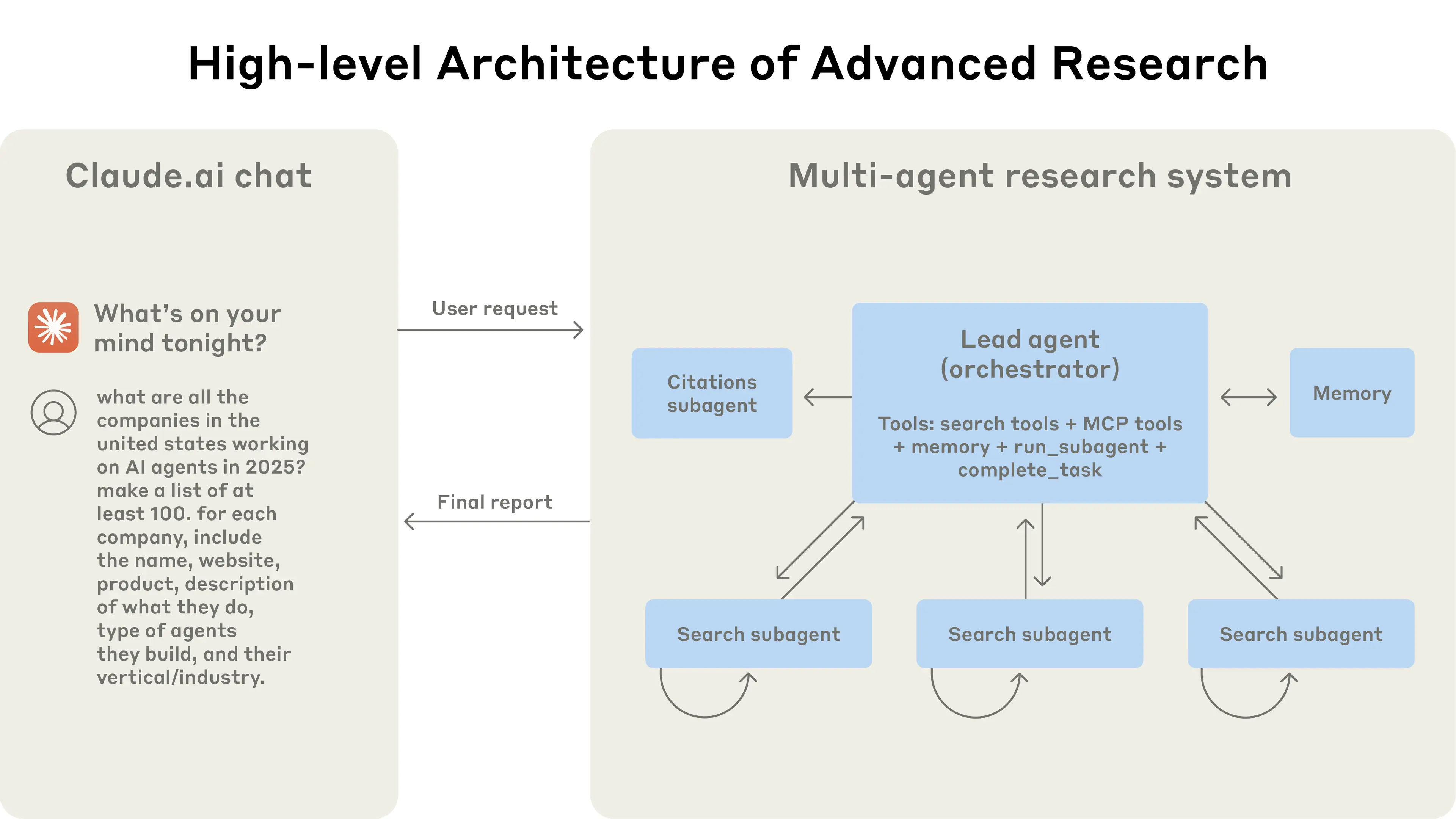
多智能体架构实际应用：用户查询通过主智能体流动，主智能体创建专门的子智能体来并行搜索不同方面。

当用户提交查询时，主智能体分析查询，制定策略，并生成子智能体来同时探索不同方面。如上图所示，子智能体作为智能过滤器，迭代使用搜索工具收集信息，在本例中是关于 2025 年的 AI 智能体公司，然后向主智能体返回公司列表，以便编制最终答案。

使用检索增强生成（RAG）的传统方法使用静态检索。也就是说，它们获取与输入查询最相似的一些块集合，并使用这些块生成响应。相比之下，我们的架构使用多步搜索，动态找到相关信息，适应新发现，并分析结果以制定高质量答案。

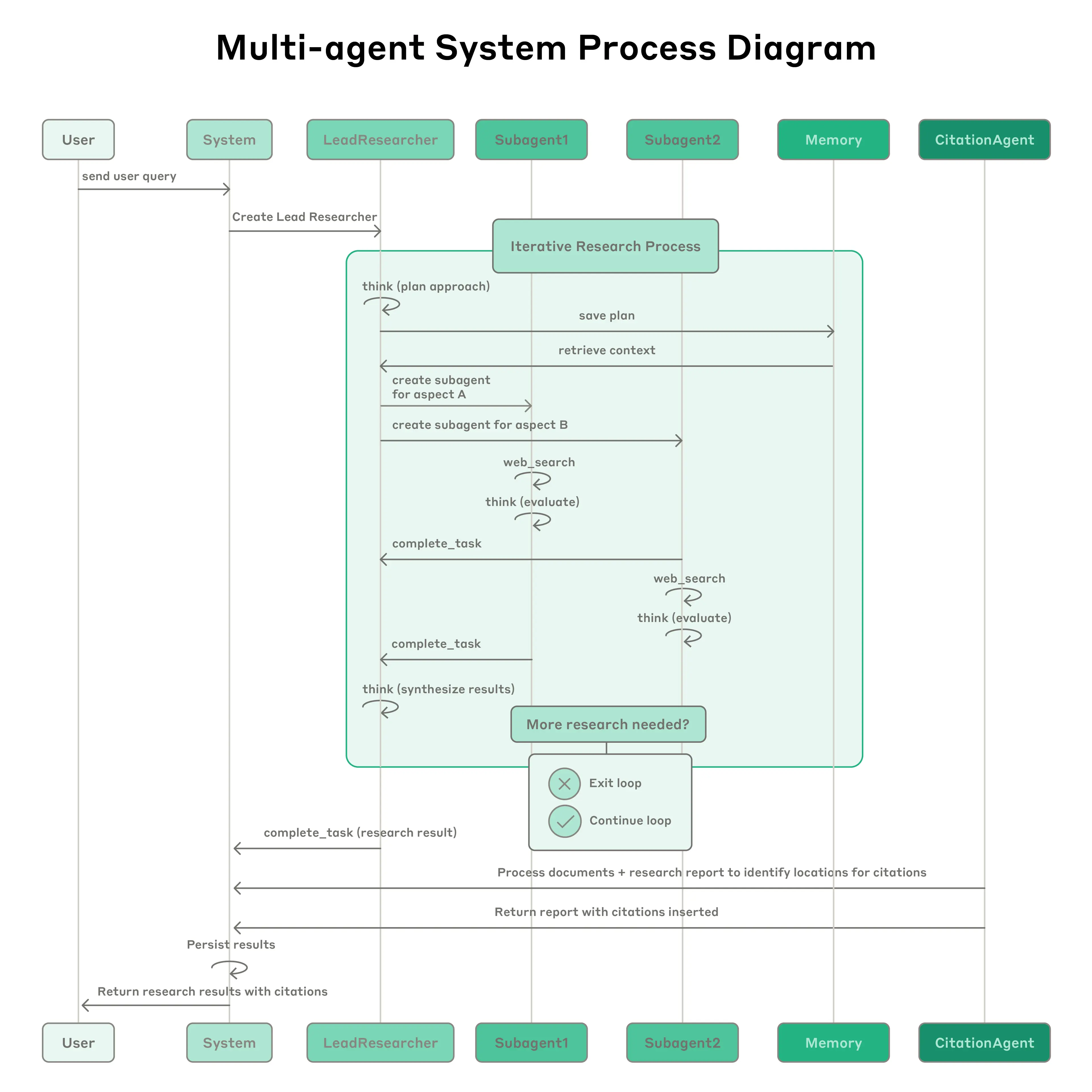
流程图显示了我们多智能体研究系统的完整工作流程。当用户提交查询时，系统创建一个 LeadResearcher 智能体，进入迭代研究过程。LeadResearcher 首先思考方法并将其计划保存到内存中以持久化上下文，因为如果上下文窗口超过 200,000 个 token，它将被截断，保留计划很重要。然后它创建具有特定研究任务的专门子智能体（这里显示了两个，但可以是任意数量）。每个子智能体独立执行网络搜索，使用交错思考评估工具结果，并将发现返回给 LeadResearcher。LeadResearcher 综合这些结果并决定是否需要更多研究——如果需要，它可以创建额外的子智能体或完善其策略。一旦收集到足够的信息，系统退出研究循环并将所有发现传递给 CitationAgent，后者处理文档和研究报告以识别引用的特定位置。这确保所有声明都正确归属于其来源。最终的研究结果，连同引用，然后返回给用户。

研究智能体的提示工程和评估

多智能体系统与单智能体系统有关键差异，包括协调复杂性的快速增长。早期智能体犯了诸如为简单查询生成 50 个子智能体、无休止地搜索不存在的来源、以及过度更新相互干扰等错误。由于每个智能体都由提示引导，提示工程是我们改善这些行为的主要杠杆。以下是我们学到的一些提示智能体的原则：

1. 像智能体一样思考

要迭代提示，你必须理解它们的效果。为了帮助我们做到这一点，我们使用来自系统的确切提示和工具，通过我们的控制台构建了模拟，然后逐步观察智能体工作。这立即揭示了故障模式：智能体在已经有足够结果时继续工作，使用过于冗长的搜索查询，或选择错误的工具。有效的提示依赖于开发智能体的准确心理模型，这可以使最有影响力的变化变得明显。

2. 教编排器如何委托

在我们的系统中，主智能体将查询分解为子任务并向子智能体描述它们。每个子智能体需要一个目标、输出格式、使用工具和来源的指导，以及明确的任务边界。没有详细的任务描述，智能体会重复工作、留下空白或无法找到必要信息。我们开始允许主智能体给出简单、简短的指令，如”研究半导体短缺”，但发现这些指令通常足够模糊，子智能体会误解任务或执行与其他智能体完全相同的搜索。例如，一个子智能体探索 2021 年汽车芯片危机，而另外两个重复工作调查当前 2025 年供应链，没有有效的分工。

3. 根据查询复杂性调整努力

智能体很难判断不同任务的适当努力，所以我们在提示中嵌入了缩放规则。简单的事实查找只需要 1 个智能体进行 3-10 次工具调用，直接比较可能需要 2-4 个子智能体，每个进行 10-15 次调用，复杂研究可能使用超过 10 个子智能体，有明确划分的责任。这些明确的指导方针帮助主智能体有效分配资源，防止在简单查询上过度投资，这是我们早期版本中的常见故障模式。

4. 工具设计和选择至关重要

智能体-工具接口与人机接口一样重要。使用正确的工具是高效的——通常，这是严格必要的。例如，智能体在网络上搜索包含学术术语的内容可能需要 Google Scholar，而不是通用网络搜索。我们设计工具时明确定义了它们的用途、限制和最佳用例。模糊的工具描述导致误用，从而产生无关结果和浪费的努力。我们还发现，为智能体提供太多工具选择可能令人困惑——策划的工具集比大量通用工具更有效。

5. 建立明确的停止条件

智能体可能会陷入无限循环，不断搜索或细化已经足够的结果。我们设置了明确的完成标准：特定数量的来源、满足的关键信息要求，或达到的时间/调用限制。我们还教智能体识别何时找到了”足够好”的答案，而不是完美的答案，这在开放性研究中经常是现实的目标。

评估多智能体系统需要新方法。传统指标如 BLEU 分数或困惑度无法捕捉复杂的多步骤研究过程的质量。我们开发了测量准确性、完整性、效率和可用性的定制评估。准确性检查智能体是否找到正确信息，完整性评估是否回答了查询的所有部分，效率测量达到结果所需的时间和资源，可用性评估最终输出对用户的有用性。

我们还发现人工评估仍然至关重要。虽然自动化指标可以大规模捕捉基本质量，但人类判断对于评估细微差别、创造性和整体实用性是不可替代的。我们的提示帮助解决了这个问题。即使在自动化评估的世界中，手动测试仍然必不可少。

多智能体系统具有涌现行为，这些行为在没有特定编程的情况下出现。例如，对主智能体的小改变可能不可预测地改变子智能体的行为方式。成功需要理解交互模式，而不仅仅是个体智能体行为。因此，这些智能体的最佳提示不仅仅是严格的指令，而是定义分工、问题解决方法和努力预算的协作框架。正确做到这一点依赖于仔细的提示和工具设计、可靠的启发式方法、可观察性和紧密的反馈循环。

生产可靠性和工程挑战

在传统软件中，错误可能破坏功能、降低性能或导致中断。在智能体系统中，微小的变化会级联成大的行为变化，这使得为必须在长时间运行过程中维护状态的复杂智能体编写代码变得非常困难。

智能体有状态且错误会复合

智能体可以长时间运行，在许多工具调用中维护状态。这意味着我们需要持久执行代码并处理沿途的错误。没有有效的缓解措施，轻微的系统故障对智能体来说可能是灾难性的。当错误发生时，我们不能只是从头开始重新启动：重新启动对用户来说是昂贵且令人沮丧的。相反，我们构建了可以从智能体发生错误时的位置恢复的系统。我们还使用模型的智能来优雅地处理问题：例如，让智能体知道工具何时失败并让它适应，效果出奇地好。我们将建立在 Claude 基础上的 AI 智能体的适应性与重试逻辑和定期检查点等确定性保障措施相结合。

调试受益于新方法

智能体做出动态决策，在运行之间是非确定性的，即使使用相同的提示。这使调试变得更困难。例如，用户会报告智能体”没有找到明显信息”，但我们看不出原因。智能体是使用糟糕的搜索查询吗？选择差的来源吗？遇到工具故障吗？添加完整的生产跟踪让我们诊断智能体失败的原因并系统性地修复问题。除了标准可观察性，我们监控智能体决策模式和交互结构——所有这些都不监控个别对话的内容，以维护用户隐私。这种高级可观察性帮助我们诊断根本原因，发现意外行为，并修复常见故障。

部署需要仔细协调

智能体系统是几乎连续运行的提示、工具和执行逻辑的高度有状态网络。这意味着每当我们部署更新时，智能体可能处于其过程中的任何位置。因此，我们需要防止我们善意的代码更改破坏现有智能体。我们不能同时将每个智能体更新到新版本。相反，我们使用彩虹部署来避免干扰运行中的智能体，通过逐渐将流量从旧版本转移到新版本，同时保持两者同时运行。

同步执行创建瓶颈

目前，我们的主智能体同步执行子智能体，等待每组子智能体完成后再继续。这简化了协调，但在智能体之间的信息流中创建了瓶颈。例如，主智能体无法引导子智能体，子智能体无法协调，整个系统可能因等待单个子智能体完成搜索而被阻塞。异步执行将实现额外的并行性：智能体并发工作并在需要时创建新的子智能体。但这种异步性在结果协调、状态一致性和跨子智能体错误传播方面增加了挑战。随着模型能够处理更长更复杂的研究任务，我们预期性能增益将证明复杂性是合理的。

结论

在构建 AI 智能体时，最后一英里通常成为大部分旅程。在开发机器上工作的代码库需要重要的工程才能成为可靠的生产系统。智能体系统中错误的复合性质意味着传统软件的小问题可能完全使智能体脱轨。一步失败可能导致智能体探索完全不同的轨迹，导致不可预测的结果。由于本文中描述的所有原因，原型和生产之间的差距通常比预期的更宽。

尽管存在这些挑战，多智能体系统已被证明对开放性研究任务有价值。用户表示 Claude 帮助他们找到了没有考虑过的商业机会，导航复杂的医疗保健选项，解决棘手的技术错误，并通过发现他们单独不会找到的研究连接节省了数天的工作。多智能体研究系统可以通过仔细的工程、全面的测试、细致的提示和工具设计、健壮的操作实践，以及对当前智能体能力有深刻理解的研究、产品和工程团队之间的紧密协作，在规模上可靠运行。我们已经看到这些系统正在改变人们解决复杂问题的方式。

人们今天使用研究功能的最常见方式。主要用例类别是：跨专业领域开发软件系统（10%），开发和优化专业和技术内容（8%），制定业务增长和收入生成策略（8%），协助学术研究和教育材料开发（7%），以及研究和验证关于人员、地点或组织的信息（5%）。

附录

以下是多智能体系统的一些额外杂项提示。

改变状态的多轮智能体的终态评估

评估在多轮对话中修改持久状态的智能体面临独特挑战。与只读研究任务不同，每个动作都可能改变后续步骤的环境，创建传统评估方法难以处理的依赖关系。我们发现专注于终态评估而不是逐轮分析是成功的。不是判断智能体是否遵循了特定过程，而是评估它是否达到了正确的最终状态。这种方法承认智能体可能找到实现相同目标的替代路径，同时仍确保它们提供预期结果。对于复杂工作流程，将评估分解为应该发生特定状态变化的离散检查点，而不是试图验证每个中间步骤。

长期对话管理

生产智能体经常参与跨越数百轮的对话，需要仔细的上下文管理策略。随着对话延长，标准上下文窗口变得不足，需要智能的压缩和内存机制。我们实施了智能体总结已完成工作阶段并在继续新任务之前将重要信息存储在外部内存中的模式。当上下文限制接近时，智能体可以通过仔细的交接生成具有干净上下文的新子智能体，同时保持连续性。此外，它们可以从内存中检索存储的上下文，如研究计划，而不是在达到上下文限制时丢失先前的工作。这种分布式方法防止上下文溢出，同时在扩展交互中保持对话连贯性。

子智能体输出到文件系统以最小化”传话游戏”

直接子智能体输出可以绕过主协调器处理某些类型的结果，提高保真度和性能。与其要求子智能体通过主智能体沟通一切，不如实施工件系统，专门智能体可以创建独立持久的输出。子智能体调用工具将其工作存储在外部系统中，然后将轻量级引用传回协调器。这防止在多阶段处理期间的信息丢失，并减少通过对话历史复制大输出的 token 开销。该模式特别适用于结构化输出，如代码、报告或数据可视化，其中子智能体的专门提示比通过通用协调器过滤产生更好的结果。

参考文献：

• 原文链接

引言

在当今的 AI 应用中，RAG 已经成为解决大语言模型知识局限性的重要技术方案。然而，构建一个高质量的 RAG 系统远不止是简单地将文档向量化后进行相似度搜索。检索环节的优化往往决定了整个系统的成败。

要保证 RAG 应用能准确检索到所需的文档，我们需要同时关注召回率（Recall）和准确率（Precision）：

• 召回率：所有相关文档中，被系统检索出来的比例
• 准确率：被系统检索出来的文档中，真正相关的比例

在 RAG 中，这两者往往是此消彼长的关系，需要找到一个最优的平衡点。

检索质量评估框架

核心指标

除了召回率和准确率，我们还需要关注以下指标：

• NDCG（Normalized Discounted Cumulative Gain）：考虑排序位置的相关性指标
• MRR（Mean Reciprocal Rank）：平均倒数排名，衡量第一个相关结果的位置
• Hit Rate@K：前 K 个结果中包含相关文档的查询比例

评估数据集构建

建立高质量的评估数据集是优化的前提。例如，对于”如何优化深度学习模型的训练速度？”这样的查询，正相关文档应该是讨论 GPU 并行、批处理优化的内容，部分相关的可能涉及模型压缩、量化，而纯理论介绍或其他领域的文档则属于不相关。

提升召回率的策略

召回率关注的是”不漏”，即尽可能地找到所有相关的文档。

1. 优化分块（Chunking）策略

分块是 RAG 的基础，而且非常重要。直接影响检索效果：

分块大小优化

• 固定大小分块：通常 512-1024 tokens 为宜。既不会太短，也不会太长。分块太小可能丢失上下文，分块太大则可能引入无关信息。
• 基于语义的动态分块：尽量按照段落、章节等自然语义边界进行分块，而不是简单的固定字符数。例如，将完整的问答对或表格作为独立的块。
• 重叠策略： 在相邻分块之间设置一定的重叠部分，有助于保留跨块的上下文信息，比如相邻块间保持 20-50 tokens 重叠。

语义边界保持

实际分块操作可能是多种分块策略结合使用。比如先基于段落进行动态分块，然后在段落内部，基于固定大一或者句子来分块。基于语义的分块策略应该考虑句子边界和语义相似度，通过句子分割、动态调整块大小、保持语义完整性等方式，确保每个分块都包含完整的语义信息。

结构化信息处理

• 表格数据：保持表格完整性，添加表头上下文。
• 代码片段：包含函数/类的完整定义。
• 列表项：保持列表的逻辑完整性。

2. 查询增强（Query Expansion）

通过扩展查询来增加召回相关文档的机会：

多角度查询生成

使用 LLM 生成多个查询变体，可以通过以下方式实现：使用同义词替换、改变句式结构、添加相关术语、简化表达、详细描述等方法，为原始查询生成多个语义相似但表达方式不同的变体。

层次化查询策略

• 粗粒度检索：使用概括性词汇扩大检索范围
• 细粒度检索：使用具体术语提高精确度
• 多层融合：综合不同粒度的检索结果

3. 混合检索（Hybrid Search）

结合多种检索方法发挥各自优势：

稀疏检索 + 密集检索

混合检索通过结合 BM25 关键词检索和向量语义检索来实现。首先分别进行两种检索，然后对检索分数进行归一化处理，最后通过加权融合（如向量检索权重 70%，BM25 权重 30%）得到最终排序结果。

多模态检索

• 文本+图像：同时索引文档中的文字和图表信息
• 结构化+非结构化：结合表格数据和自然语言描述
• 元数据增强：利用时间、作者、类别等元信息

提升准确率的策略

准确率关注的是”不瞎”，即召回的文档都是真正需要的。

1. 嵌入模型优化

嵌入模型质量直接决定向量检索的准确性：

领域适配

• 预训练模型选择：如科学文献使用 SciBERT，法律文档使用 LegalBERT
• 微调策略：在特定领域数据上进行对比学习微调
• 多语言支持：针对中英文混合文档的特殊处理

嵌入维度优化

嵌入维度的选择需要在性能和质量之间找平衡：

• 128 维：速度快、准确率低、内存占用小
• 384 维：速度中等、准确率中等、内存占用中等
• 768 维：速度慢、准确率高、内存占用大
• 1024 维：速度很慢、准确率很高、内存占用很大

2. 重排序（Reranking）

对初始检索结果进行精细化排序：

Cross-Encoder 重排序

使用重排序模型对候选文档进行精细排序的过程包括：构建查询-文档对、使用重排序模型计算相关性分数、根据分数进行排序，最终返回排序后的前 K 个文档。

多阶段重排序

1. 粗排：使用轻量级模型快速筛选Top-100
2. 精排：使用复杂模型对Top-20进行精确排序
3. 多样性调整：避免结果过于集中在相似文档

3. 智能过滤策略

预过滤机制

• 元数据过滤：根据文档类型、时间范围、权威性筛选
• 关键词门槛：确保文档包含查询的核心术语
• 质量评分：基于文档完整性、可读性的预评分

后过滤优化

检索后的文档过滤包括多个层面：相关性阈值过滤（如最低相关性 0.3）、重复内容检测（如相似度阈值 0.8）、内容质量检查等，通过这些过滤机制确保最终返回的文档都符合质量要求。

高级优化技术

1. 自适应检索策略

根据查询特征动态调整检索策略。首先分析查询的复杂度特征，然后根据不同类型采用相应策略：简单查询重点使用关键词匹配，概念性查询重点进行语义理解，复杂查询则采用混合策略。

2. 查询意图理解

意图分类

• 事实查询：寻找具体信息（who, what, when）
• 程序查询：寻找操作步骤（how to）
• 比较查询：对比不同选项（difference, comparison）
• 分析查询：深入理解（why, analysis）

针对性优化

根据不同查询意图采用相应的优化策略：

• 事实查询：embedding 权重 30%，关键词权重 70%，使用事实聚焦的重排序模型
• 程序查询：embedding 权重 60%，关键词权重 40%，使用步骤感知的重排序模型
• 分析查询：embedding 权重 80%，关键词权重 20%，使用上下文感知的重排序模型

3. 动态索引优化

增量更新策略

• 热点文档：高频访问文档的索引优化
• 时效性文档：新增文档的快速索引
• 过期清理：定期清理不再相关的文档

索引压缩技术

• 向量量化：使用PQ（Product Quantization）压缩
• 稀疏化：去除低权重的向量维度
• 分层索引：构建粗粒度到细粒度的多层索引

实践中的平衡之道

召回优先策略

在实际应用中，通常采用”召回优先，精度优化”的两阶段策略：

1. 广泛召回阶段

   • 使用宽松的相似度阈值
   • 应用多种查询扩展技术
   • 结合多种检索方法

2. 精度优化阶段

   • 应用重排序模型
   • 执行多层过滤
   • 进行结果去重和多样性优化

性能与质量权衡

不同应用场景需要不同的配置策略：

• 实时问答：延迟预算 <200ms，采用轻量级 embedding+简单重排序，牺牲部分准确率换取响应速度
• 深度分析：延迟预算 <5s，采用高质量 embedding+复杂重排序，容忍较高延迟获得最佳质量
• 批量处理：无延迟限制，采用多模型 ensemble+全面后处理，追求最高质量

持续优化机制

A/B 测试框架

• 检索策略对比：不同算法的效果验证
• 参数调优：阈值、权重等超参数优化
• 用户体验监控：基于真实反馈的持续改进

监控指标体系

建立全面的监控指标体系：

• 检索质量：NDCG@10、MRR、Hit Rate@5
• 系统性能：平均延迟、P99 延迟、QPS
• 用户满意度：点击率、停留时间、反馈评分
• 业务指标：任务完成率、准确答案比例、用户留存

未来发展趋势

1. 多模态检索融合

随着多模态大模型的发展，RAG 系统将更好地处理文本、图像、音视频等多种模态的信息检索和融合。

2. 个性化检索优化

基于用户历史行为和偏好，构建个性化的检索模型，提供更精准的个人知识服务。

3. 实时学习能力

检索系统将具备从用户反馈中实时学习的能力，持续优化检索质量。

总结

RAG 系统的检索优化是一个系统性工程，需要从分块策略、查询处理、检索算法、重排序等多个维度进行综合优化。关键在于：

1. 建立完善的评估体系：确保优化方向正确
2. 平衡召回率与准确率：根据应用场景找到最优平衡点
3. 采用分层优化策略：粗排+精排的两阶段设计
4. 持续监控和迭代：基于真实数据不断优化

只有通过系统性的优化和持续的迭代改进，才能构建出既能全面检索，又能精准定位的高质量 RAG 应用，为用户提供准确、及时、有价值的信息服务。

本文将深入探讨为什么分块如此重要，以及如何通过几种核心策略来优化它。

什么是词块

将词块视为 RAG 系统中知识的原子单元 。每个词块应该：

• 语义完整 ：包含单独来看有意义的连贯信息。
• 语境丰富 ：包含足够的周围环境，无需外部参考即可理解。
• 最佳尺寸 ：足够大以具有意义，足够小以便精确检索。
• 边界感知 ：尊重句子、段落和章节等自然语言结构。

这些要求经常相互冲突。语义完整的块可能太大，无法进行精确检索。大小合适的块可能会在边界处丢失关键上下文。这时，不同的分块策略就派上用场了。每种方法都有各自的优缺点，最佳选择取决于您的具体用例、文档类型和检索需求。

分块策略

下面由浅入深，介绍不同的分块策略：

固定大小分块（简单基线）

固定大小分块将文档拆分为预定大小的块，通常以以下方式测量：

• 字符数 （例如，每块 1000 个字符）
• 令牌数量 （例如，每块 256 个令牌）
• 字数统计 （例如，每段 200 个字）

重叠参数在这里至关重要。如果没有重叠，您可能会丢失跨越块边界的信息。重叠率为 20% 时，可以确保相邻块之间有一定的连续性。

固定大小分块策略几乎不适用于任何场景，仅在有限计算资源的情况。固定大小分块适用的场景：

• 有统一、简单的文档（博客、文章、小说）
• 处理速度至关重要
• 存储和计算资源严重有限

语义分块

语义分块代表着思维的根本性转变。语义分块不再根据大小限制任意切割文本，而是根据语义和文档结构识别自然断点。语义分块需要更多的计算资源，但能带来更好的结果。

核心见解：文档具有固有的语义边界，可以指导分块决策。

语义分块的工作原理：

1. 句子分割 ：将文档分解成单个句子
2. 嵌入生成 ：为每个句子创建向量表示
3. 相似度分析 ：测量相邻句子之间的语义相似度
4. 边界检测 ：在相似度低于阈值的地方创建块边界
5. 组块 ：将连续相似的句子组合成连贯的组块

高级语义技术：

• 主题建模集成 ：使用基于 LDA 或 BERT 的主题模型来识别主题边界
• 层次聚类 ：在分块之前按语义相似度对句子进行分组
• 实体连续性 ：确保命名实体及其引用保持在同一块内
• 话语标记 ：使用语言线索（但是、此外、总之）来识别界限

语义分块适用于很多场景：

• 文档质量差异很大
• 上下文保存很重要
• 准确性比速度更重要

分层文档分块

对于具有嵌套结构的复杂文档（例如技术手册、法律合同或学术论文），分层分块可以保留文档的组织逻辑。这种方法认识到文档不是平面文本，而是具有章节、小节和逻辑层次的结构化知识。

分层分块的主要优点：

• 上下文继承 ：每个块都知道它在文档层次结构中的位置
• 元数据保存 ：维护章节标题、级别和关系
• 结构感知检索 ：您可以按不同的粒度进行检索（部分与小节）
• 交叉引用处理 ：对其他部分的引用仍然有意义

对于 200 页的技术手册，分层分块可能会创建：

1. 15 个章节级块（高级概述）
2. 127 个部分级块（详细解释）
3. 340 个子节级块（具体程序）

在检索过程中，系统可以将查询与适当的细节级别进行匹配，并提供分层上下文。

如果出现以下情况，则实施分层分块：

• 文件结构清晰（手册、报告、学术论文）
• 用户需要不同程度的细节
• 交叉引用很常见
• 文档格式结构良好

滑动窗口分块（重叠优化器）

传统的组块方法会创建离散的、不重叠的组块。但是，如果最重要的信息恰好落在组块边界上，该怎么办呢？滑动窗口分块通过创建重叠块解决了这个问题，确保没有信息被遗漏。

当 window_size=1000、stride=800 时，可获得 200 个字符的重叠（20%）。此重叠可确保：

1. 关键句子没有被拆分成多个部分
2. 上下文在相邻块之间自然流动
3. 检索有多次机会找到相关信息

自适应滑动窗口

高级实现根据内容密度调整窗口大小和步幅：

1. 常见问题解答文档 ：问题和答案受益于重叠的上下文
2. 法律文件 ：精确的语言界限至关重要
3. 技术程序 ：步骤参考先前的操作
4. 叙事内容 ：故事连续性至关重要

大模型分块

使用大语言模型进行递归分块： 最新的进展是使用 LLM 本身进行分块决策。

多模态分块

对于包含图像、表格和混合内容的文档。

基于查询模式的动态分块

最先进的系统根据文档的实际查询方式来调整分块。

Agent 设计范式

目前主流的 AI Agent（智能体）设计模式，通常不是单一的，而是基于一些核心思想和框架的组合。这些设计模式旨在赋予大语言模型自主思考、规划、行动和反思的能力，以完成更复杂的任务。

1. ReAct (Reasoning and Acting)

这是目前最流行、最基础也是最核心的一种 Agent 设计模式。它的核心思想是让大语言模型在一个“思考-行动-观察”的循环中持续工作，直到任务完成。

• 思考（Thought）：LLM 会根据当前任务和过往观察，产生一段内部思考，比如“我需要找到XX信息，我应该使用什么工具？”
• 行动（Action）：LLM 根据思考，生成一个调用外部工具的指令（即 Function Call）。
• 观察（Observation）：LLM 接收到外部工具返回的结果。

这个循环会反复进行，直到 LLM 判断任务已完成并生成最终回复。这种模式将”思考”过程显性化，使得模型的决策过程更加透明和可控。

2. Plan-and-Execute（规划与执行）

这种模式更侧重于对复杂任务的结构化分解。它将一个大任务分为两个阶段：

• 规划阶段（Planning）：LLM 首先会分析用户的请求，并生成一个详细的、分步骤的行动计划。这个计划是固定的，不会在执行过程中轻易改变。
• 执行阶段（Execution）：LLM 严格按照规划好的步骤，一步一步地调用工具和执行任务。

这种模式的优点是任务流程清晰、稳定，适合需要按部就班完成的复杂任务。但缺点是缺乏灵活性，如果计划中的某个步骤失败，Agent 可能无法自主调整。

3. Self-Correction（自我纠正/反思）

这种设计模式的核心是让 Agent 具备复盘和纠错的能力。它通常与其他模式结合使用，为 Agent 增加一个”反思”步骤。

• 反思（Reflection）：Agent 在完成一个任务或得到一个结果后，会重新评估这个结果是否正确或达到预期。
• 纠正（Correction）：如果评估结果不理想，Agent 会根据反思结果，修改其原始的思考路径或行动计划，然后再次尝试，直到达到满意的结果。

这种模式能显著提升 Agent 在复杂问题上的表现，因为它允许 Agent 从错误中学习，避免重复犯错。

这三种模式并不是相互独立的。一个强大的 Agent 通常会结合使用这些思想：例如，一个 Agent 可能先用 Plan-and-Execute 进行任务分解，然后在每个执行步骤中，使用 ReAct 循环来调用工具，并最终用 Self-Correction 机制来验证和修正结果。

大模型如何”用”工具？Agent、Function Call 与 MCP 的进化之路

在构建基于大语言模型（LLM）的应用时，一个核心挑战是让 LLM 不只停留在”聊天”，而是真正具备”行动”能力，比如联网搜索、调用 API 或执行代码。这就是 Agent 的核心思想：让 LLM 像一个智能体一样，能够根据用户的指令，自主决定是直接回答，还是调用外部工具来获取信息或完成任务。

1. Agent 的决策过程：LLM 如何知道何时调用工具？

Agent 的决策机制本质上是 Prompt Engineering 的一种高级应用。开发者会设计一个精巧的 Prompt，将可用的工具列表、它们的用途和描述一并告诉 LLM。

例如，当我们问一个 Agent：“今天北京的天气怎么样？”它的思考过程可能如下：

1. 用户意图分析： 用户想知道北京的天气。
2. 工具匹配： 我有一个可以查询天气的工具（get_weather(location)）。
3. 决策与执行： 我需要调用这个工具，并把“北京”作为参数。

这个思考过程并不神秘，而是通过精心设计的 Prompt 来引导 LLM 生成。LLM 会根据输入的指令和工具描述，在输出中”思考”并生成一个结构化的行动指令，然后由外部程序（Agent 框架）去实际执行。

2. Function Call (FC)：将决策能力内置到模型中

Function Call (FC) 是对上述 Agent 决策机制的一种原生优化。它将“思考”和“生成调用指令”的能力直接通过模型训练内置进去。

FC 的核心是： 模型能够根据上下文，直接以预先定义好的 JSON 格式 生成对外部工具的调用，而不是像传统 Agent 那样需要外部框架去解析 LLM 生成的文本。

这是一种巨大的进步，因为它使得工具调用更加稳定、高效，并减少了外部解析的复杂性。

那么，为什么说 FC 存在“MxN”的问题？

这里有一个常见的误解：很多人以为每增加一个工具，就需要重新训练模型。这是不正确的。

FC 的”MxN”问题不在于模型本身，而在于 工具的描述格式。每个拥有 FC 能力的 LLM 平台（如 OpenAI, Google, Anthropic）都有自己独特的工具描述 Schema（函数签名）。一个搜索工具，为了能被不同的模型调用，开发者需要为它编写 M 份不同的描述文档。同样，一个 Agent 开发者如果想使用 N 个工具，并支持 M 个不同的 LLM，就需要处理 MxN 个兼容性问题。

简而言之，FC 解决了“让模型知道如何调用工具”的问题，但没有解决“工具描述格式不统一”的问题。

3. MCP：通过抽象层实现真正的解耦

Multi-tool Coordinator Protocol (MCP) 正是为了解决 FC 带来的兼容性与扩展性问题而诞生的。

MCP 的核心思想是：在模型和工具之间增加一个抽象的中间层。

这个中间层通常由一个 MCP Server 组成，其工作流程如下：

1. 工具注册： 所有外部工具都按照一套统一的 MCP 协议 接入并注册到 MCP Server。
2. Agent (LLM) 接入： 所有的 Agent 只需要学习并支持这套统一的 MCP 协议。它们不再需要知道每个工具的具体描述细节，只需向 MCP Server 发送一个统一的请求，来获取可用的工具列表或执行工具调用。

为什么说 MCP 实现了“M+N”？

• M 个不同的模型（或 Agent）只需要对接 1 个统一的 MCP Server。
• N 个不同的工具也只需要对接 1 个统一的 MCP Server。

通过这种方式，模型与工具之间不再是复杂的点对点连接，而是通过一个中心化的枢纽进行通信。这不仅解决了 FC 在不同平台间的兼容性问题，更是一种架构上的巨大优化，它让工具的管理、维护和扩展变得前所未有的简单。

总结来说：

• Agent 是让 LLM 具备行动能力的 思想。
• Function Call 是将这种思想 内置到模型中 的一种能力。
• MCP 是在此基础上，进一步将 模型与工具解耦 的一种 架构设计。

当然，MCP 还需要在调用端封装。在典型的 MCP (Multi-tool Coordinator Protocol) 实现中，会区分 AI Host (AI 宿主) 和 MCP Client (MCP 客户端) 这两个角色，它们通过一种清晰的协作模式来共同完成任务。

1. AI Host (AI 宿主)

   • 角色： AI Host 是整个系统的核心，通常是运行大语言模型（LLM）或 Agent 框架的那部分。它负责接收用户的指令，并进行高级别的决策与推理。
   • 职责：
     • 接收用户输入。
     • 与 LLM 交互，进行意图分析。
     • 根据 LLM 的输出，决定是直接生成回复还是需要调用工具。
     • 注意： AI Host 不直接与具体的工具交互，它只知道 MCP 协议。

2. MCP Client (MCP 客户端)

   • 角色： MCP Client 是一个独立的模块或库，作为 AI Host 与 MCP Server 之间的桥梁。它封装了所有与 MCP Server 通信的细节。
   • 职责：
     • 将来自 AI Host 的工具调用请求，按照 MCP 协议 进行格式化，并发送给 MCP Server。
     • 接收 MCP Server 返回的结果，并将其转换回 AI Host 可理解的格式。
     • 管理与 MCP Server 的连接和会话。
     • 注意： MCP Client 也不关心具体的工具是如何实现的，它只负责协议层面的通信。

整个 MCP 协作过程可以分解为以下几个步骤：

1. 用户请求： 用户向 AI Host 发出指令，例如：“帮我查一下旧金山的天气。”
2. AI Host 意图分析： AI Host 将用户指令发送给内置的 LLM。LLM 基于其 Function Call 或 ReAct 能力，判断出需要调用一个天气查询工具。它会生成一个结构化的调用请求，比如 {"tool_name": "weather_api", "parameters": {"city": "旧金山"}}。
3. AI Host 委托： AI Host 拿到 LLM 生成的调用请求后，并不会自己去执行，而是将其 委托 给 MCP Client。
4. MCP Client 协议转换与发送： MCP Client 接收到这个请求，将其封装成符合 MCP 协议的格式（例如一个特定的 HTTP POST 请求或 gRPC 调用），然后发送给远端的 MCP Server。
5. MCP Server 工具协调与执行： MCP Server 接收到请求后，根据 tool_name 找到对应的工具，将 parameters 传递给该工具并执行。
6. 结果返回： 工具执行完毕，结果返回给 MCP Server，MCP Server 再将结果通过 MCP 协议返回给 MCP Client。
7. MCP Client 结果转换与回传： MCP Client 接收到 MCP Server 的响应，将其解析并转换为 AI Host 可理解的格式，然后返回给 AI Host。
8. AI Host 回复生成： AI Host 拿到工具执行结果（例如：”旧金山今天多云，气温 15 摄氏度”），将其作为上下文的一部分再次输入给 LLM，最终由 LLM 生成完整的自然语言回复给用户。

通过这种方式，AI Host 始终保持”干净”，只关心高级别的推理和决策，而具体的工具调用和协议通信的复杂性则完全由 MCP Client 和 MCP Server 这层抽象来处理，实现了 AI 能力与工具生态的彻底解耦。

最后，通过一个图说明 FC 和 MCP 工作模式：

JSON 格式化输出

在 Function Call (FC) 模式下，要保证模型稳定输出 JSON 格式，主要依赖于 模型本身的训练和微调。

如何保证模型稳定输出 JSON？

这并非单纯通过 Prompt Engineering 就能完美解决的问题。核心在于：

1. 大规模训练： 在模型的预训练和指令微调阶段，会使用大量的包含 JSON 格式的结构化数据作为训练样本。这些样本告诉模型，当它接收到特定类型的指令（例如，要求它调用某个工具）时，应该输出一个遵循特定 JSON Schema 的结果。
2. 特殊的解码策略： 一些模型在解码时会采用特殊的约束，比如 JSON Schema 约束解码。这意味着，模型在生成每一个 token 时，都会检查其是否符合预先定义的 JSON 格式规则。如果生成的 token 会导致 JSON 格式无效，模型会将其“回溯”并尝试生成另一个 token，直到生成完整且正确的 JSON。这种方法极大地提高了输出的稳定性和正确性。
3. Prompt 工程辅助： 尽管核心能力来自模型本身，但好的 Prompt 仍然至关重要。例如，在 Prompt 中清晰地描述工具的函数签名，并明确要求模型“请以 JSON 格式输出调用结果”，可以进一步引导模型输出期望的格式。

比如这个 FC 输出的格式：

1
2
3
4
5
6
7

{
  "name": "get_current_weather",
  "arguments": {
    "location": "旧金山",
    "unit": "celsius"
  }
}

其中的每个 key 和 value 都要非常精准的匹配到调用的工具才可以。

MCP 是否也要求模型输出固定格式？

是的，但要求的是更简单、更统一的格式。

MCP 的核心理念是 解耦。它将工具的复杂性和多样性从模型端剥离，因此模型不需要了解每个工具具体的 JSON Schema。模型唯一需要知道的，是与 MCP Client 交互的 统一协议。

这个统一协议的格式通常非常简单，比如一个包含 tool_name 和 parameters 的 JSON 对象。模型需要做的，只是稳定输出这个简单的、所有工具都通用的 JSON 格式，然后由 MCP Client 去处理后续的协议转换和工具调用。

这正是 MCP 的优势所在：它降低了对模型的要求。模型不需要针对每一个新工具去学习其独特的调用格式，它只需要掌握一套通用的、简单的输出格式即可。这使得模型可以更专注于其核心的自然语言理解和意图识别，而将复杂的
工具协调任务交给 MCP Client 和 MCP Server 去完成。

下面是一个模型输出的 MCP 格式的调用：

1
2
3
4
5
6
7

{
  "tool_name": "weather_api",
  "parameters": {
    "city": "旧金山",
    "temp_unit": "celsius"
  }
}

这个看起来比较类似，但实际上模型并不知道 weather_api 到底是什么，也不知道对于一个 city，应该传入的参数是什么（city？location？），对于温度单位，也类似。

FC (Function Call) 模式下，模型的难度体现在 “量” 上。模型需要记忆并理解每一个工具独特的 JSON Schema，而且要非常精确。如果你的系统有 100 个不同的工具，每个工具的参数都不一样，那模型就需要稳定地输出 100 种不同结构的 JSON。这就像让一个人记住 100 个完全不同的表格格式，并根据指令填写。

而 MCP (Multi-tool Coordinator Protocol) 模式下，模型的难度只体现在 “质” 上。它只需要学会一种 统一且简单的 JSON 格式，即 {“tool_name”: “…”, “parameters”: {…}}。无论有多少个工具，这个输出格式始终不变。这就像让一个人永远只填写一种固定格式的表格，然后把表格交给一个“总机”去处理后续的细节。

MCP Client 拿到的模型输出，也就是通用且简单的 JSON 格式（例如：{“tool_name”: “…”, “parameters”: {…}}），负责将其解析、封装、调用 Server、接收响应、解析响应，回传给 AI Host。

引言

随着大语言模型规模的快速增长，显存需求呈指数级增长。传统的分布式训练方法虽然能够利用多 GPU 进行训练，但每个 GPU 仍然需要存储完整的模型参数、梯度和优化器状态，这严重限制了可训练的模型规模。

ZeRO 技术通过数据并行与内存优化的结合，将模型训练中的大块数据（优化器状态、梯度和模型参数）分散到不同的 GPU 上，而非在每个 GPU 上都完整存储一份，从而显著降低了每个 GPU 的显存需求。

ZeRO 技术原理

传统数据并行的问题

在传统的数据并行训练中，每个 GPU 都需要存储：

1. 模型参数：完整的模型权重
2. 梯度：完整的梯度信息
3. 优化器状态：如 Adam 优化器的动量、方差等状态

对于大规模模型，这些数据占用的显存非常庞大。例如，一个 175B 参数的模型使用 Adam 优化器时，仅优化器状态就需要约 700GB 显存（每个参数需要 4 个 float32 值）。

ZeRO 的核心思想

ZeRO 的核心思想是消除冗余存储，通过分片技术将原本每个 GPU 都需要存储的完整数据分散到多个 GPU 上，实现显存的线性扩展。

关键洞察：

• 在数据并行中，不同 GPU 上的模型参数是相同的
• 梯度在反向传播后需要进行 All-Reduce 操作
• 优化器状态与参数一一对应

基于这些观察，ZeRO 提出了分阶段的内存优化策略。

ZeRO 的三个阶段

ZeRO-Stage 1：优化器状态分片（Optimizer State Sharding）

原理：
将优化器状态分片存储在不同的 GPU 上，每个 GPU 只存储部分优化器状态。

具体做法：

• 假设有 $N$ 个 GPU，模型参数为 $P$
• 将优化器状态分成 $N$ 个分片，每个 GPU 存储 $P/N$ 个参数对应的优化器状态
• 在参数更新时，每个 GPU 只更新自己负责的那部分参数

内存节省：

• 优化器状态内存减少 $N$ 倍
• 对于 Adam 优化器，每个参数需要 4 个 float32 值，节省效果显著

ZeRO-Stage 2：梯度分片（Gradient Sharding）

原理：
在 Stage 1 的基础上，进一步将梯度分片存储。

具体做法：

• 每个 GPU 只计算和存储部分梯度
• 在反向传播结束时，通过 All-Reduce 操作收集完整的梯度
• 然后每个 GPU 只更新自己负责的参数部分

内存节省：

• 梯度内存减少 $N$ 倍
• 与 Stage 1 结合，总内存节省更加显著

ZeRO-Stage 3：参数分片（Parameter Sharding）

原理：
在 Stage 1 和 Stage 2 的基础上，进一步将模型参数分片存储。

具体做法：

• 模型参数也被分片存储在不同的 GPU 上
• 在训练过程中，当需要某个层的所有参数时，通过 All-Gather 操作将所需参数动态地收集到当前 GPU
• 这意味着在任何给定时间点，每个 GPU 上只完整存在模型参数的一部分

内存节省：

• 模型参数内存减少 $N$ 倍
• 实现了最大程度的内存优化

ZeRO 的具体实现

通信模式

ZeRO 使用了两种主要的通信模式：

1. All-Gather：用于参数收集

   • 当需要某个层的完整参数时，从所有 GPU 收集该层的参数分片
   • 通信开销：$O(P)$，其中 $P$ 是参数数量

2. All-Reduce：用于梯度聚合

   • 在反向传播后，聚合所有 GPU 上的梯度分片
   • 通信开销：$O(P)$

内存管理策略

按需加载机制：

• 参数只在需要时才加载到 GPU 显存
• 使用完毕后立即释放，避免长期占用显存

分片存储策略：

• 优化器状态：静态分片，训练过程中保持不变
• 梯度：动态分片，每次反向传播后重新分配
• 参数：动态分片，根据计算需求动态加载

计算流程

前向传播：

1. 通过 All-Gather 收集当前层需要的参数
2. 执行前向计算
3. 释放不需要的参数

反向传播：

1. 通过 All-Gather 收集当前层需要的参数
2. 计算梯度
3. 将梯度分片存储
4. 释放参数

参数更新：

1. 通过 All-Reduce 聚合所有梯度分片
2. 每个 GPU 更新自己负责的参数部分
3. 更新对应的优化器状态

ZeRO 的变体技术

ZeRO-Offload

原理：
对于模型训练中一些对性能不那么敏感，但内存占用大的部分（如优化器状态、甚至梯度），将其从 GPU 显存转移到 CPU 内存或硬盘（NVMe SSD）。

具体做法：

• 优化器状态存储在 CPU 内存中
• 梯度可以存储在 CPU 内存或 NVMe SSD 中
• 在需要时通过 PCIe 总线传输数据

优势：

• 进一步减少 GPU 显存需求
• 能够训练更大的模型
• 成本相对较低

劣势：

• 增加了 CPU-GPU 数据传输开销
• 训练速度可能有所下降

ZeRO-FSDP（Fully Sharded Data Parallelism）

原理：
ZeRO-FSDP 是 ZeRO-Stage 3 的完整实现，实现了优化器状态、梯度和模型参数的全面分片。

特点：

• 最大程度的内存优化
• 支持任意大小的模型训练
• 通信开销相对较高

GRPO 算法概述

在 LLM 的 RLHF 训练中，PPO 虽然表现良好，但仍存在一些可以改进的地方：

1. GAE 的复杂性：PPO 使用 GAE 计算每个 token 的优势，涉及多个超参数（$\lambda$、$\gamma$）的调优
2. 价值函数的需求：PPO 需要训练一个 Critic 模型来估计状态价值，增加计算和内存成本
3. 训练不稳定：在某些场景下，GAE 估计的方差仍然较大，导致训练波动

GRPO 通过一个更直接的方法来解决这些问题：将序列级的奖励直接分配到 token 级别，然后通过组内相对比较来计算优势。这种方法在实践中被证明更加稳定高效。

GRPO 的核心创新：

1. 简化优势计算：不使用 GAE，而是通过组内相对奖励直接计算优势
2. 减少计算负担：虽然仍需要参考模型，但优势计算逻辑更简洁
3. 提高训练稳定性：通过序列奖励的分解和组内比较，减少方差
4. Token 级别的精细控制：在每个 token 级别进行重要性采样和裁剪

GRPO 的动机

GRPO 相比 PPO 的改进方向：

GRPO 的三个核心模型

与 PPO 不同，GRPO 只需要三个模型：

关键区别：GRPO 相比 PPO 不需要 Critic 模型，这大大减少了训练的计算和内存成本。

GRPO 的算法原理

1. 序列奖励的分解

GRPO 的核心创新是如何将序列级的奖励分配到token 级别。

奖励分配机制

对于长度为 $T$ 的生成序列，Reward Model 给出一个标量奖励 $r_{\text{RM}}$。GRPO 将这个奖励分配到每个 token：

即：只有最后一个 token（序列终止位置）获得奖励，中间所有 token 的奖励为 0。

这与 PPO 中的 KL 惩罚方式不同（PPO 中每个 token 都有 $-\beta \log \frac{\pi_\theta}{\pi_{\text{ref}}}$ 的惩罚）。

为什么这样分配

• 简洁性：不需要为每个 token 计算即时奖励和 KL 惩罚的组合
• 合理性：反映了现实情况——我们只在完整回答后评分
• 直观性：整个序列的质量用一个数字衡量，然后均等分配（或按距离衰减）

2. Token 级别的重要性采样与裁剪

这是 GRPO 与 PPO 最重要的区别之一。

PPO 的做法（token 级别）

PPO 对每个 token 计算重要性采样比率：

然后进行裁剪和加权：

特点：重要性采样是 token 级别的，优势 $A_t$ 也是 token 级别的。

GRPO 的做法（仍是 token 级别，但优势不同）

GRPO 同样对每个 token 计算重要性采样比率：

然后进行裁剪和加权：

其中 $\tilde{A}_t$ 是 token 级别的归一化优势（见下一节）。

重要：GRPO 仍然是 token 级别的重要性采样和裁剪，但优势的计算方式不同。

3. 组内相对优势计算

这是 GRPO 最核心的创新。

序列优势（第一步）

对于生成的每个序列 $i$，根据其奖励计算序列级优势：

其中：

• $r_i$：第 $i$ 个序列的 RM 奖励
• $\bar{r} = \frac{1}{G} \sum_{j=1}^{G} r_j$：组内（所有 $G$ 个序列）的平均奖励

含义：这个序列相对于组内平均水平的相对优势。

Token 级优势（第二步）

GRPO 将序列优势分配给序列中的每个 token。最简单的做法是均等分配：

其中 $T_i$ 是第 $i$ 个序列的长度。

也可以使用折扣分配（越靠近末端权重越高）：

其中 $\gamma \in [0,1]$ 是折扣因子（通常 0.99）。折扣分配的好处是给予序列末端（生成过程的最后）更高的权重，这更符合直觉：序列的最后部分对最终质量影响更大。

优势归一化

为了稳定训练，对组内的优势进行归一化：

其中：

• $\mu_A = \frac{1}{G \cdot T} \sum_i \sum_t \tilde{A}_t^{(i)}$：所有 token 优势的平均值
• $\sigma_A$：所有 token 优势的标准差
• $\epsilon$：小常数防止除零

4. 完整的损失函数

GRPO 的损失函数包含两部分：

策略损失

或者使用 PPO 风格的裁剪：

KL 约束损失

注意：GRPO 仍然保留 KL 约束，防止策略偏离参考模型太远。

GRPO 与 PPO 的详细对比

模型架构对比

优势计算对比

重要性采样对比

关键相同点：GRPO 和 PPO 都在 token 级别进行重要性采样和裁剪，区别在于优势的计算来源。

优缺点对比

PPO 的优势

1. 原理清晰：基于价值函数的强化学习理论
2. 广泛应用：在各种 RL 任务中都有良好表现
3. 灵活性强：可以适应各种奖励结构
4. 理论支持：GAE 有深厚的理论基础

PPO 的缺陷

1. 模型多：需要训练两个大模型（Actor + Critic）
2. Critic 不准确：Critic 的价值估计可能不准确，导致优势估计有偏差
3. 超参数多：GAE 的 $\lambda, \gamma$ 需要调优
4. 计算成本高：训练 Critic 占用显存和计算力

GRPO 的优势

1. 模型少：无需额外训练 Critic，只需 Actor
2. 方差小：组内比较天然降低方差，不依赖模型准确性
3. 简洁直接：优势计算逻辑简单明了
4. 计算成本低：节省 Critic 的计算和内存

GRPO 的缺陷

1. 需要分组：必须采样一个组的序列，组大小 $G$ 需要调优
2. 依赖组质量：如果组内所有序列都很差，相对优势可能无法有效指导
3. 序列奖励稀疏：不能充分利用中间步骤的反馈信息
4. 较少应用：目前应用不如 PPO 广泛

GRPO 的实现细节

1. 分组采样

GRPO 的关键是在每次更新时采样一个组的序列。

采样策略

1. 输入：一个 batch 的 prompts，共 $B$ 个
2. 采样：对每个 prompt，采样 $G$ 个序列（即 $G$ 个不同的回答）
3. 结果：得到 $B \times G$ 个序列

组大小选择

• $G = 4$：计算效率高，但相对优势估计可能不够准确
• $G = 8 \sim 16$：平衡效率和准确性（推荐）
• $G = 32$：优势估计准确，但计算成本大

实践建议：根据显存和计算资源选择，通常 $G = 8$ 或 $G = 16$。

2. 奖励获取与归一化

奖励获取流程

对每个序列：

1. Actor 生成：Actor 生成完整序列
2. RM 评分：将序列输入 RM，得到标量奖励 $r_{\text{RM}}$
3. 记录：保存奖励值

奖励归一化

1
2
3
4
5
6

# 对每个 prompt 的 G 个序列的奖励进行归一化
for prompt_idx in range(B):
    rewards = [r[prompt_idx, :] for r in reward_scores]  # G 个奖励
    mu = np.mean(rewards)
    sigma = np.std(rewards)
    normalized_rewards = (rewards - mu) / (sigma + 1e-8)

为什么归一化：

• 不同的 prompt 可能有不同的奖励尺度
• 归一化后的优势在 0 附近，梯度更稳定

3. Token 优势计算

算法步骤

对于第 $i$ 个序列（长度 $T_i$，奖励 $r_i$）：

步骤 1：计算序列优势

步骤 2：分配到每个 token（选择一种）

方式 A：均等分配

方式 B：折扣分配

步骤 3：全局归一化

Python 伪代码

1
2
3
4
5
6
7
8
9
10
11
12
13
14
15
16
17
18
19
20
21
22
23
24
25
26
27
28
29
30
31
32
33
34
35
36
37
38
39
40
41

def compute_advantages(rewards, sequence_lengths, discount=0.99):
    """
    Args:
        rewards: shape (B, G) - B 个 prompts，每个 G 个序列的奖励
        sequence_lengths: shape (B, G) - 每个序列的长度
        discount: 折扣因子
    
    Returns:
        advantages: shape (B, G, T_max) - 每个 token 的优势
    """
    B, G, T_max = rewards.shape[0], rewards.shape[1], sequence_lengths.max()
    
    # 全局平均奖励
    global_mean = rewards.mean()
    
    # 序列优势
    seq_advantages = rewards - global_mean  # shape (B, G)
    
    # token 级优势（折扣分配）
    token_advantages = np.zeros((B, G, T_max))
    
    for b in range(B):
        for g in range(G):
            T = sequence_lengths[b, g]
            A_seq = seq_advantages[b, g]
            
            # 计算折扣和
            discount_sum = sum(discount**(T-1-t) for t in range(T))
            
            # 分配到每个 token
            for t in range(T):
                token_advantages[b, g, t] = (
                    discount**(T-1-t) * A_seq / discount_sum
                )
    
    # 全局归一化
    mean_adv = token_advantages.mean()
    std_adv = token_advantages.std()
    normalized_advantages = (token_advantages - mean_adv) / (std_adv + 1e-8)
    
    return normalized_advantages

4. 损失计算与反向传播

Token 级别的损失计算

对于第 $i$ 个序列的第 $t$ 个 token：

重要性采样比率：

PPO 风格的裁剪损失：

其中 $\epsilon = 0.2$（裁剪范围）。

KL 约束

计算方式（对于语言模型）：

在实际实现中，通常只计算被生成 token 处的 KL：

总体损失

单个序列的损失（先 token 后序列平均）：

整个组的损失（序列平均）：

Python 伪代码

1
2
3
4
5
6
7
8
9
10
11
12
13
14
15
16
17
18
19
20
21
22
23
24
25
26
27
28
29
30
31
32
33
34
35
36
37
38
39

def compute_loss(logits, reference_logits, advantages, token_ids, beta=0.05, epsilon=0.2):
    """
    Args:
        logits: shape (B, G, T, V) - Actor 模型输出
        reference_logits: shape (B, G, T, V) - Reference 模型输出
        advantages: shape (B, G, T) - 归一化优势
        token_ids: shape (B, G, T) - 生成的 token IDs
        beta: KL 权重
        epsilon: 裁剪范围
    
    Returns:
        loss: 标量损失
    """
    B, G, T, V = logits.shape
    
    # 计算 log 概率
    log_probs = log_softmax(logits, dim=-1)  # shape (B, G, T, V)
    ref_log_probs = log_softmax(reference_logits, dim=-1)
    
    # 选择生成 token 的概率
    chosen_log_probs = log_probs.gather(-1, token_ids.unsqueeze(-1)).squeeze(-1)
    chosen_ref_log_probs = ref_log_probs.gather(-1, token_ids.unsqueeze(-1)).squeeze(-1)
    
    # 重要性采样比率
    log_ratio = chosen_log_probs - chosen_ref_log_probs  # log(pi/pi_ref)
    ratio = exp(log_ratio)  # pi/pi_ref
    
    # PPO 裁剪损失
    clipped_ratio = clamp(ratio, 1 - epsilon, 1 + epsilon)
    policy_loss = -min(ratio * advantages, clipped_ratio * advantages)
    
    # KL 散度（简化版，只计算生成的 token）
    kl_loss = log_ratio  # 近似
    
    # 总损失
    total_loss = policy_loss + beta * kl_loss
    
    # 求平均
    return total_loss.mean()

5. 超参数设置

关键超参数

调优建议

1. $G$ 的选择：

   • 显存充足：使用 $G = 16$ 或更大
   • 显存紧张：使用 $G = 4$ 或 $G = 8$
   • 避免 $G$ 过小（$< 4$），否则相对优势不可靠

2. $\beta$ 的调优：

   • 若 KL 散度过大：增大 $\beta$
   • 若训练不动（模型变化太慢）：减小 $\beta$
   • 推荐从 $0.05$ 开始，根据 KL 散度监测值调整

3. 学习率的选择：

   • GRPO 的学习率通常比 SFT 小 100-1000 倍
   • 从 5e-7 开始，根据梯度范数调整
   • 避免学习率过大，否则训练不稳定

4. 折扣因子 $\gamma$：

   • $\gamma = 0.99$：末端 token 权重约为前端的 $0.37$ 倍
   • $\gamma = 1.0$：均等分配（最简单）
   • 推荐从 $\gamma = 1.0$ 开始，必要时调整

GRPO 的完整训练流程

算法伪代码

1
2
3
4
5
6
7
8
9
10
11
12
13
14
15
16
17
18
19
20
21
22
23
24
25
26
27
28
29
30
31
32
33
34
35
36
37
38
39
40
41
42
43
44
45
46
47
48
49

算法：GRPO 训练

初始化：
  - Actor 模型 π_θ（可以从 SFT 初始化）
  - Reference 模型 π_ref（冻结，使用 SFT 模型或 Actor 的检查点）
  - Reward Model R（冻结，提前训练）

主循环：
  for epoch = 1 to num_epochs:
    for batch_idx = 1 to num_batches:
      
      # 步骤 1: 采样
      prompts = get_batch()  # B 个 prompts
      sequences = []
      log_probs = []
      
      for g = 1 to G:
        # 使用 Actor 生成 G 个回答
        seq_g, logprobs_g = generate_from_actor(prompts, π_θ)
        sequences.append(seq_g)
        log_probs.append(logprobs_g)
      
      # 步骤 2: 获取奖励
      rewards = reward_model.score(sequences)  # shape (B, G)
      
      # 步骤 3: 计算优势
      advantages = compute_advantages(rewards, sequences)  # shape (B, G, T)
      
      # 步骤 4: 前向传播
      actor_outputs = actor(sequences)  # 获取 Actor 的 logits
      ref_outputs = reference_model(sequences)  # 获取 Reference 的 logits
      
      # 步骤 5: 计算损失
      loss = 0
      for each token:
        ratio = exp(log_pi_theta - log_pi_ref)
        clipped_ratio = clip(ratio, 1-ε, 1+ε)
        policy_loss += min(ratio * A, clipped_ratio * A)
        kl_loss += (log_pi_theta - log_pi_ref)
      
      total_loss = policy_loss + β * kl_loss
      
      # 步骤 6: 反向传播和更新
      optimizer.zero_grad()
      total_loss.backward()
      optimizer.step()
      
      # 步骤 7: 监测
      log(loss, kl_div, reward_mean, reward_std)

训练流程图

1
2
3
4
5
6
7
8
9
10
11
12
13
14
15
16
17
18
19
20
21
22
23
24
25
26
27
28
29
30
31
32
33
34
35
36
37
38
39
40
41
42

┌─────────────────────────────────────────────────────┐
│ 输入：Batch of Prompts                               │
└─────────────────────┬───────────────────────────────┘
                      ↓
            ┌─────────────────────┐
            │ Actor 采样 G 个序列  │  （并行，每个 prompt）
            └──────────┬──────────┘
                       ↓
      ┌────────────────────────────────┐
      │ Reward Model 评分每个序列       │
      │ 得到 (B, G) 的奖励矩阵         │
      └────────────┬───────────────────┘
                   ↓
      ┌────────────────────────────────┐
      │ 计算序列优势（组内相对比较）   │
      │ A_i^seq = r_i - mean(r)        │
      └────────────┬───────────────────┘
                   ↓
      ┌────────────────────────────────┐
      │ 分配到 Token 级优势             │
      │ A_t = discount^(T-t) * A_seq   │
      └────────────┬───────────────────┘
                   ↓
      ┌────────────────────────────────┐
      │ 全局归一化优势                 │
      │ A_hat = (A - mean) / std       │
      └────────────┬───────────────────┘
                   ↓
      ┌────────────────────────────────┐
      │ 计算 PPO 损失（token 级别）    │
      │ L = min(r*A, clip(r)*A)        │
      │ + β * KL(π_θ || π_ref)        │
      └────────────┬───────────────────┘
                   ↓
      ┌────────────────────────────────┐
      │ 反向传播和梯度更新             │
      │ θ ← θ - α ∇L                   │
      └────────────┬───────────────────┘
                   ↓
            ┌──────────────────┐
            │ 输出：更新的 Actor │
            └──────────────────┘

GRPO 完整数值示例

让我们用一个具体例子演示整个计算过程。

假设条件

• 批大小：$B = 1$（1 个 prompt）
• 组大小：$G = 2$（2 个序列）
• 序列长度：$T_1 = 3, T_2 = 4$（两个序列长度不同）
• 奖励：$r_1 = 0.8, r_2 = 0.6$（第一个序列更好）
• 折扣因子：$\gamma = 0.99$
• 裁剪范围：$\epsilon = 0.2$
• KL 权重：$\beta = 0.05$

计算过程

步骤 1: 计算序列优势

1
2
3
4
5
6
7
8

序列 1: r_1 = 0.8, T_1 = 3
序列 2: r_2 = 0.6, T_2 = 4

平均奖励: r_bar = (0.8 + 0.6) / 2 = 0.7

序列优势:
  A_1^seq = 0.8 - 0.7 = 0.1
  A_2^seq = 0.6 - 0.7 = -0.1

解释：序列 1 相对于平均水平好一点，序列 2 相对于平均水平差一点。

步骤 2: 分配到 Token 级（使用折扣分配）

折扣分配公式：

其中分母是折扣权重的和。

序列 1 计算（$T_1 = 3$）：

1
2
3
4
5
6

折扣权重: γ^(3-1)=0.9801, γ^(3-2)=0.99, γ^(3-3)=1.0
权重和: 0.9801 + 0.99 + 1.0 = 2.9701

Token 1: A_1^(1) = (0.9801 * 0.1) / 2.9701 = 0.0330
Token 2: A_2^(1) = (0.99 * 0.1) / 2.9701 = 0.0333
Token 3: A_3^(1) = (1.0 * 0.1) / 2.9701 = 0.0337

序列 2 计算（$T_2 = 4$）：

1
2
3
4
5
6
7

折扣权重: γ^(4-1)=0.9703, γ^(4-2)=0.9801, γ^(4-3)=0.99, γ^(4-4)=1.0
权重和: 0.9703 + 0.9801 + 0.99 + 1.0 = 3.9404

Token 1: A_1^(2) = (0.9703 * (-0.1)) / 3.9404 = -0.0246
Token 2: A_2^(2) = (0.9801 * (-0.1)) / 3.9404 = -0.0249
Token 3: A_3^(2) = (0.99 * (-0.1)) / 3.9404 = -0.0251
Token 4: A_4^(2) = (1.0 * (-0.1)) / 3.9404 = -0.0254

观察：

• 序列 1 的最后 token (0.0337) 权重高于最前 token (0.0330)
• 序列 2 的所有优势都是负的（因为序列质量较差）

步骤 3: 全局归一化

所有 token 的优势值：

1
2
3
4
5
6
7
8
9

序列 1: [0.0330, 0.0333, 0.0337]
序列 2: [-0.0246, -0.0249, -0.0251, -0.0254]

合并: [0.0330, 0.0333, 0.0337, -0.0246, -0.0249, -0.0251, -0.0254]

均值: μ_A = (0.0330 + 0.0333 + 0.0337 - 0.0246 - 0.0249 - 0.0251 - 0.0254) / 7
           = 0 / 7 = 0 (近似)

方差: σ_A ≈ 0.0291

归一化后（减去均值、除以标准差）：

1
2

序列 1: [0.1134, 0.1145, 0.1159]  (正值，鼓励)
序列 2: [-0.0846, -0.0856, -0.0863, -0.0873]  (负值，惩罚)

步骤 4: 计算 PPO 损失

假设 Actor 和 Reference 模型在序列 1 的第 1 个 token 处：

• Actor log_prob: -1.5
• Reference log_prob: -1.6
• 生成的 token ID

计算过程：

1
2
3
4
5
6
7
8
9
10

log_ratio = -1.5 - (-1.6) = 0.1
ratio = exp(0.1) ≈ 1.105

优势: A_hat_1^(1) = 0.1134

无裁剪: ratio * A_hat = 1.105 * 0.1134 ≈ 0.1253
有裁剪: clip(ratio, 0.8, 1.2) = 1.105
        clipped * A_hat = 1.105 * 0.1134 ≈ 0.1253

PPO loss: min(0.1253, 0.1253) = 0.1253

步骤 5: KL 散度

假设 KL 散度计算（简化）：

1
2
3
4
5

KL_1^(1) = log_ratio = 0.1

总 KL 损失 (简化，仅示意):
L_KL = β * log_ratio_sum / num_tokens
     = 0.05 * (所有 log_ratio 之和) / 7

最终损失

1
2
3
4

序列 1 损失: L_1 = (L_policy_1 + β * L_KL_1) / 3
序列 2 损失: L_2 = (L_policy_2 + β * L_KL_2) / 4

总损失: L = (L_1 + L_2) / 2

关键观察：

• 序列 1 的优势为正，鼓励增加这些 token 的概率
• 序列 2 的优势为负，抑制这些 token 的概率
• Token 级别的优势差异（末端 > 前端）反映了对最终质量的贡献

GRPO 的收敛性与稳定性

方差分析

GRPO 相比 PPO 的方差优势来自于：

1. 组内相对比较：

   • PPO 使用单个序列的价值函数差分 $\delta_t$，仅与该序列相关
   • GRPO 使用组内所有序列的平均，$E[\text{Var}(A_t)]$ 更小

2. 不依赖模型准确性：

   • PPO 的 GAE 依赖 Critic 的准确性
   • GRPO 直接使用真实奖励，无模型误差

3. 折扣分配的效果：

   • 给予末端更高权重，减少信号的不确定性

收敛性证明

GRPO 的收敛性可以通过以下论证：

1. 策略改进：每次更新时，$\mathbb{E}[r_t A_t] \geq 0$ 当 $A_t > 0$
2. KL 约束限制：防止策略离开信任域（trust region）
3. 优势无偏估计：组内比较提供无偏的相对信号

定理（简化版）：在合理的假设下，GRPO 的策略序列收敛到满足 KL 约束的最优策略。

GRPO 在实践中的表现

DeepSeek 的实验结果

根据 DeepSeek 的研究报告，GRPO 在以下指标上表现出色：

数学推理任务（GSM8K/MATH）

• 收敛速度：更快（通常 10-50% 的步数）
• 最终效果：相当或优于 PPO（特别是在数学问题上）
• 训练稳定性：更稳定，奖励波动更小

通用能力（基准测试）

• 不会显著退化：通过 KL 约束保持基础能力
• 任务特定性强：在目标任务上显著改进，日常闲聊改进不大
• 内存节省：相比 PPO 节省 20-30% 的显存（无需 Critic）

什么情况下 GRPO 更好

1. 有明确的 RM 评分：任务有定量的奖励信号（数学、代码、写作评分等）
2. 大规模模型：模型越大，Critic 的省省成本越显著
3. 单轮生成：适合生成单个长序列的场景（如数学推导、代码）

GRPO 可能不如 PPO 的情况

1. 奖励信号不清晰：RM 评分方差大、不稳定
2. 组大小受限：显存不足，无法采样足够大的组
3. 多步交互任务：需要按步骤获得反馈的任务

常见问题与解答

Q1: GRPO 是否需要参考模型？

A: 是的。GRPO 需要参考模型来计算 KL 约束，防止策略漂移。虽然 GRPO 不需要 Critic，但仍需要 Reference 模型（通常是 SFT 模型的冻结副本）。

Q2: GRPO 的组大小 G 应该怎么选？

A:

• 最小值：$G \geq 4$（否则相对优势不可靠）
• 推荐值：$G = 8 \sim 16$（平衡准确性和效率）
• 最大值：受显存限制，通常 $G \leq 32$

根据经验，$G$ 增加一倍通常能稍微改进效果但计算成本翻倍。

Q3: GRPO 会过度拟合组内序列吗？

A: 有可能。如果组大小 $G$ 太小，相对优势的估计可能不稳定。解决方案：

1. 增加 $G$ 的大小
2. 跨 batch 计算优势（不仅限于单个 batch 内的序列）
3. 加入额外的正则化

Q4: GRPO 的 KL 散度约束怎么调？

A: 观察 KL 散度的值：

• 若 KL > 0.1：$\beta$ 太小，增大 $\beta$
• 若 KL < 0.01：$\beta$ 太大，减小 $\beta$
• 目标范围：0.01-0.05

Q5: GRPO vs PPO，我应该选哪个？

A: 根据以下决策树：

1
2
3
4
5
6
7
8
9
10
11
12

计算资源充足？
  ├─ 是 → PPO（通用性强，理论支持好）
  └─ 否 → GRPO（节省 Critic 显存）

任务类型？
  ├─ 数学/代码 → GRPO 可能更好
  ├─ 通用闲聊 → PPO 或 GRPO 都可
  └─ 多步交互 → PPO 更安全

显存约束是否严格？
  ├─ 是 → GRPO
  └─ 否 → PPO 或 GRPO

总结

GRPO 代表了 LLM RLHF 训练的一个重要方向，其核心贡献包括：

1. 简化优势计算：从复杂的 GAE 到简单的组内相对比较
2. 减少计算负担：不需要额外的 Critic 模型
3. 提高稳定性：组内比较天然降低方差
4. 实用高效：在大规模模型上表现更好

关键理解：

• GRPO 仍然是 token 级别的重要性采样和裁剪（与 PPO 相同）
• GRPO 的创新在于优势的计算方式（组内相对而非 GAE）
• GRPO 和 PPO 是互补的方法，根据具体场景选择

推荐阅读：

• Efficient Stage-wise Pretraining for Large Language Models (GRPO 原论文)
• 配合 PPO 博文 理解两种算法的异同

引言

在大语言模型的推理过程中，生成式推理（Generative Inference）是一个自回归过程，模型需要逐个生成token。在这个过程中，大量的计算被重复执行，特别是Attention机制中的Key和Value矩阵计算。KV Cache技术通过缓存这些中间结果，避免了重复计算，从而显著提高了推理效率。

本文将详细介绍KV Cache的工作原理，从Attention计算的数学原理出发，推导其等价性，并分析其在实际应用中的优化效果。

Attention机制回顾

标准Attention计算

在Transformer的Attention机制中，对于输入序列 $X = [x_1, x_2, …, x_n]$，Attention的计算过程如下：

1. 线性变换

其中：

• $W_Q, W_K, W_V$ 是查询、键、值的权重矩阵
• $Q, K, V$ 分别是查询、键、值的矩阵表示

2. Attention计算

其中 $d_k$ 是键向量的维度。

3. 分步展开
对于第 $i$ 个位置的输出，可以表示为：

其中：

自回归生成过程

在生成式推理中，模型逐个生成token。假设当前已经生成了 $t$ 个token，要生成第 $t+1$ 个token：

输入序列：$X_{1:t} = [x_1, x_2, …, x_t]$

计算过程：

1. 计算 $Q{1:t}, K{1:t}, V_{1:t}$
2. 计算Attention输出
3. 生成下一个token $x_{t+1}$
4. 重复上述过程

问题：每次生成新token时，都需要重新计算整个序列的 $K$ 和 $V$ 矩阵，这导致了大量的重复计算。

KV Cache的核心思想

基本概念

KV Cache的核心思想是：缓存已经计算过的Key和Value矩阵，避免重复计算。

缓存内容：

• $K_{cache} = [K_1, K_2, …, K_t]$：已生成token的Key矩阵
• $V_{cache} = [V_1, V_2, …, V_t]$：已生成token的Value矩阵

增量更新：

• 生成新token $x{t+1}$ 时，只计算 $K{t+1}$ 和 $V_{t+1}$
• 将新的Key和Value追加到缓存中
• 使用完整的缓存进行Attention计算

数学等价性推导

1. 标准计算的数学表示

在标准计算中，生成第 $t+1$ 个token时：

输入：$X{1:t+1} = [x_1, x_2, …, x_t, x{t+1}]$

计算过程：

Attention输出：

其中：

2. KV Cache的计算表示

在KV Cache中，生成第 $t+1$ 个token时：

缓存状态：

• $K_{cache} = [K_1, K_2, …, K_t]$
• $V_{cache} = [V_1, V_2, …, V_t]$

增量计算：

更新缓存：

Attention计算：

其中：

这里注意重点，$O{t+1}$，只和 $\alpha{(t+1)j}$ 以及 $v{i:t+1}$ 有关。而 $\alpha{(t+1)j}$ 只和 $q{t+1}$ 以及 $k{i:t+1}$ 有关，这也是为何需要 KV 缓存，而不需要 Q 缓存的原因。这是 Attention 计算的核心，也是实现 KV cache 的关键。

3. 等价性证明

矩阵运算的线性性质：

对于线性变换 $K = XW_K$，由于矩阵乘法的线性性质：

同理：

Attention计算的等价性：

在标准计算中：

在KV Cache中：

由于：

• $[K{cache}, k{t+1}] = K_{1:t+1}$
• $[V{cache}, v{t+1}] = V_{1:t+1}$
• $q{t+1}$ 是 $Q{1:t+1}$ 的最后一行

因此，两种计算方式在数学上完全等价。

计算复杂度分析

1. 标准计算复杂度

第 $t+1$ 步的计算量：

• 线性变换：$O((t+1) \times d_{model} \times d_k)$
• Attention计算：$O((t+1)^2 \times d_k)$
• 总复杂度：$O((t+1) \times d_{model} \times d_k + (t+1)^2 \times d_k)$

累积计算量（生成 $n$ 个token）：

2. KV Cache计算复杂度

第 $t+1$ 步的计算量：

• 线性变换：$O(d_{model} \times d_k)$（只计算新token）
• Attention计算：$O((t+1)^2 \times d_k)$
• 总复杂度：$O(d_{model} \times d_k + (t+1)^2 \times d_k)$

累积计算量（生成 $n$ 个token）：

3. 优化效果

计算量减少：

• 线性变换部分：从 $O(n^2 \times d{model} \times d_k)$ 减少到 $O(n \times d{model} \times d_k)$
• 减少比例：$O(n)$ 倍

实际效果：

• 对于长序列生成，计算量减少显著
• 特别是在生成较长文本时，优化效果明显

KV Cache的实现细节

内存管理

1. 缓存结构

缓存格式：

1
2
3
4
5

# 缓存结构示例
kv_cache = {
    'key': torch.zeros(seq_len, num_layers, num_heads, head_dim),
    'value': torch.zeros(seq_len, num_layers, num_heads, head_dim)
}

内存布局：

• 按层（layer）组织
• 每层包含多个注意力头（attention heads）
• 支持动态扩展

2. 内存优化策略

预分配策略：

• 根据最大序列长度预分配内存
• 避免频繁的内存重新分配

内存复用：

• 在推理过程中复用缓存空间
• 减少内存碎片

增量更新机制

1. 缓存更新

更新流程：

1. 计算新token的Key和Value
2. 将新的Key和Value追加到缓存
3. 更新缓存的有效长度

代码示例：

1
2
3
4

def update_kv_cache(kv_cache, new_k, new_v, layer_idx):
    # 追加新的Key和Value到缓存
    kv_cache['key'][layer_idx] = torch.cat([kv_cache['key'][layer_idx], new_k], dim=0)
    kv_cache['value'][layer_idx] = torch.cat([kv_cache['value'][layer_idx], new_v], dim=0)

2. 注意力计算

使用缓存的Attention计算：

1
2
3
4
5
6
7
8
9
10
11
12

def attention_with_cache(query, kv_cache, layer_idx):
    # 获取缓存的Key和Value
    cached_k = kv_cache['key'][layer_idx]
    cached_v = kv_cache['value'][layer_idx]
    
    # 计算注意力分数
    scores = torch.matmul(query, cached_k.transpose(-2, -1)) / math.sqrt(d_k)
    attention_weights = torch.softmax(scores, dim=-1)
    
    # 计算输出
    output = torch.matmul(attention_weights, cached_v)
    return output

多头注意力处理

1. 多头并行计算

缓存组织：

• 每个注意力头独立缓存Key和Value
• 支持并行计算

计算优化：

1
2
3
4
5
6
7
8
9
10
11
12
13
14

def multi_head_attention_with_cache(query, kv_cache, layer_idx):
    batch_size, num_heads, seq_len, head_dim = query.shape
    
    # 并行计算所有注意力头
    outputs = []
    for head_idx in range(num_heads):
        head_query = query[:, head_idx, :, :]
        head_k = kv_cache['key'][layer_idx][:, head_idx, :, :]
        head_v = kv_cache['value'][layer_idx][:, head_idx, :, :]
        
        head_output = attention_with_cache(head_query, head_k, head_v)
        outputs.append(head_output)
    
    return torch.cat(outputs, dim=1)

2. 内存布局优化

连续内存布局：

• 将多头数据存储在连续内存中
• 提高缓存命中率

批处理优化：

• 支持批量处理多个序列
• 减少内存访问开销

引言

在当今的信息检索领域，随着人工智能和自然语言处理技术的发展，文本检索技术已经从传统的基于关键词匹配的方法，发展到了基于深度学习的语义检索方法。文本检索是RAG（Retrieval-Augmented Generation）系统的核心组件，它负责从大规模文档集合中检索出与用户查询最相关的文档片段，为后续的生成模型提供上下文信息。

本文将详细介绍三种主要的文本检索方法：稠密向量检索（Dense Retrieval）、稀疏向量检索（Sparse Retrieval）和BM25算法，以及它们的混合使用策略。

稠密向量检索（Dense Retrieval）

稠密向量检索的基本原理

稠密向量检索是一种基于深度学习的检索方法，它通过将文本转换为高维空间中的连续向量表示，然后使用向量相似度（如余弦相似度、欧氏距离）来检索相关文档。

核心思想：

• 将查询和文档都映射到同一个高维向量空间
• 通过计算向量间的相似度来衡量相关性
• 能够捕捉文本的深层语义信息

技术实现

1. 文本编码

稠密向量检索通常使用预训练的语言模型（如BERT、T5、Sentence-BERT等）对文本进行编码：

其中：

• $\mathbf{q}$ 是查询的向量表示
• $\mathbf{d}$ 是文档的向量表示
• $\text{Encoder}$ 是预训练的语言模型

2. 相似度计算

常用的相似度计算方法包括：

余弦相似度：

点积相似度：

欧氏距离：

3. 索引和检索

向量索引：

• 使用FAISS、Annoy、HNSW等向量索引库
• 支持高效的近似最近邻搜索
• 能够处理百万级别的向量检索

检索流程：

1. 将查询编码为向量
2. 在向量索引中搜索最相似的文档向量
3. 返回相似度最高的文档

稠密向量检索的优势和局限性

优势：

1. 语义理解能力强：能够理解查询和文档的深层语义
2. 处理同义词和近义词：即使词汇不完全匹配，也能找到相关文档
3. 支持复杂查询：能够处理自然语言形式的查询

局限性：

1. 计算成本高：需要深度学习模型进行编码
2. 索引规模限制：在大规模数据集上可能遇到性能瓶颈
3. 对训练数据敏感：检索效果依赖于编码模型的训练质量

应用场景

• 智能问答系统：从知识库中检索相关答案
• 推荐系统：基于内容相似性推荐相关文档
• 语义搜索：理解用户意图的搜索引擎

稀疏向量检索（Sparse Retrieval）

稀疏向量检索的基本原理

稀疏向量检索是基于传统信息检索模型的方法，它使用词袋模型（Bag of Words）将文本表示为稀疏向量，并通过计算词频-逆文档频率（TF-IDF）来评估文档与查询的相关性。

核心思想：

• 将文本表示为高维稀疏向量
• 每个维度对应词汇表中的一个词
• 通过统计方法计算词的重要性

技术实现

1. TF-IDF计算

词频（Term Frequency, TF）：

逆文档频率（Inverse Document Frequency, IDF）：

TF-IDF权重：

2. 向量构建

文档向量 $\mathbf{d}$ 的构建：

其中 $t_1, t_2, …, t_n$ 是词汇表中的所有词。

3. 相似度计算

余弦相似度：

点积相似度：

稀疏向量检索的优势和局限性

优势：

1. 计算效率高：基于统计方法，计算速度快
2. 可解释性强：能够明确知道哪些词贡献了相关性
3. 处理大规模数据：能够高效处理大规模文档集合

局限性：

1. 语义理解能力弱：无法处理同义词和近义词
2. 词汇匹配限制：需要查询词在文档中实际出现
3. 无法处理语义相似性：无法理解词汇的深层含义

应用场景

• 传统搜索引擎：基于关键词的网页搜索
• 文档检索系统：从文档库中检索相关文档
• 信息过滤：基于关键词的信息过滤

BM25算法

BM25算法的基本原理

BM25（Best Matching 25）是一种经典的信息检索算法，它是TF-IDF算法的改进版，通过引入词频（TF）和文档频率（DF）的函数来计算文档与查询的相关性得分。

核心思想：

• 在TF-IDF基础上引入文档长度归一化
• 使用词频饱和函数处理高频词
• 通过参数调整优化检索效果

数学公式

BM25算法的核心公式：

其中：

• $Q$ 是查询，包含词 $q_1, q_2, …, q_n$
• $D$ 是文档
• $f(q_i, D)$ 是词 $q_i$ 在文档 $D$ 中的词频
• $|D|$ 是文档 $D$ 的长度
• $\text{avgdl}$ 是文档集合的平均长度
• $k_1$ 和 $b$ 是调节参数

IDF计算：

其中：

• $N$ 是文档集合的总文档数
• $n(q_i)$ 是包含词 $q_i$ 的文档数

参数调节

$k_1$ 参数：

• 控制词频饱和程度
• 通常设置为 1.2-2.0
• 值越大，词频的影响越线性

$b$ 参数：

• 控制文档长度归一化程度
• 取值范围为 0-1
• $b=0$ 表示不进行长度归一化
• $b=1$ 表示完全归一化

BM25算法的优势

1. 理论基础扎实：基于概率检索模型
2. 参数可调节：能够适应不同的数据集和需求
3. 计算效率高：基于统计方法，计算速度快
4. 效果稳定：在许多基准测试中表现优异

应用场景

• 搜索引擎：Google、Bing等搜索引擎的核心算法
• 文档检索：企业文档管理系统
• 学术搜索：学术论文检索系统

混合检索策略

混合检索的基本原理

混合检索结合了稠密向量检索、稀疏向量检索和BM25算法的优势，通过多路召回和结果融合来提高检索系统的整体性能。

核心思想：

• 使用多种检索方法并行检索
• 通过融合算法合并检索结果
• 平衡准确性和召回率

混合检索的优势

1. 互补性：不同方法各有优势，相互补充
2. 提高准确性：通过多路召回提高检索准确性
3. 提升召回率：增加检索结果的覆盖面
4. 适应性：能够适应不同的查询类型和场景

实现方法

1. 多路召回

稠密向量检索：

• 使用语义相似性进行检索
• 适合处理语义相关的查询

稀疏向量检索：

• 使用关键词匹配进行检索
• 适合处理精确匹配的查询

BM25检索：

• 使用传统信息检索方法
• 适合处理结构化查询

2. 结果融合

RRF（Reciprocal Rank Fusion）：

其中：

• $\text{rank}_i(d)$ 是文档 $d$ 在第 $i$ 个检索方法中的排名
• $k$ 是调节参数，通常设置为 60

加权融合：

其中：

• $w_i$ 是第 $i$ 个检索方法的权重
• $\text{score}_i(d)$ 是文档 $d$ 在第 $i$ 个检索方法中的得分

3. 动态权重调整

根据查询类型动态调整不同检索方法的权重：

• 语义查询：增加稠密向量检索的权重
• 关键词查询：增加稀疏向量检索和BM25的权重
• 混合查询：平衡各种方法的权重

系统架构

查询处理层：

• 查询解析和预处理
• 查询类型识别
• 参数选择

检索层：

• 多路并行检索
• 结果初步排序
• 去重和合并

融合层：

• 结果融合算法
• 最终排序
• 结果返回

性能评估指标

检索性能指标

准确率（Precision）：

召回率（Recall）：

F1分数：

平均精度（MAP）：

其中 $\text{AP}(q)$ 是查询 $q$ 的平均精度。

效率指标

检索延迟：从查询到返回结果的时间
吞吐量：单位时间内处理的查询数
索引大小：索引占用的存储空间

实际应用中的优化策略

索引优化

倒排索引：

• 为每个词建立文档列表
• 支持快速的关键词查找
• 优化存储和查询效率

向量索引：

• 使用HNSW、IVF等算法
• 支持高效的近似最近邻搜索
• 平衡精度和速度

查询优化

查询扩展：

• 使用同义词扩展查询
• 基于用户反馈调整查询
• 利用查询日志优化

查询重写：

• 将自然语言查询转换为结构化查询
• 使用查询模板提高效率
• 基于历史查询进行优化

缓存策略

结果缓存：

• 缓存热门查询的结果
• 使用LRU等策略管理缓存
• 提高响应速度

索引缓存：

• 将常用索引加载到内存
• 使用分层缓存策略
• 优化内存使用

引言

大语言模型（LLM）在近年来取得了巨大的成功，但同时也面临着两个关键问题：幻觉（Hallucination）和重复（Repetition）。这些问题不仅影响了模型的实用性，也阻碍了其在关键领域的应用。本文将从底层机理出发，深入分析这两个问题的成因，并探讨有效的解决方案。

幻觉问题（Hallucination）

幻觉的基本概念

幻觉是指LLM生成的内容与事实不符，包括：

• 事实性幻觉：生成错误的事实信息。
• 逻辑性幻觉：推理过程存在逻辑错误，前后矛盾不一致。
• 指令性幻觉：指令遵循不一致，比如要求用英语回答，用中文回答。

幻觉产生的底层机理

1. 训练数据质量问题

数据噪声与错误

• 训练数据中本身就包含错误信息
• 网络爬取的数据质量参差不齐
• 标注错误导致模型学习到错误的知识

数据分布偏差

• 某些领域的数据过于稀少
• 时间性信息过时（如2023年之前的数据）
• 地域性偏见导致知识覆盖不均

2. Attention机制的局限性

根据Attention理论，Attention机制本质上是一个2体相互作用系统：

其中：

• $\mathbf{N}^{(0)}$ 是上下文向量
• $\mathsf{W}_V$ 是Value投影矩阵
• $\mathbf{x}$ 是词汇表中的token

Attention机制的固有问题：

1. 局部性限制：Attention主要关注局部相关性，难以捕捉全局一致性
2. 缺乏事实验证：模型无法验证生成内容的真实性
3. 过度依赖训练数据：当遇到训练数据中未覆盖的情况时，容易产生幻觉

3. 训练目标与事实性不匹配

最大似然估计的局限性

• 训练目标是最小化预测下一个token的损失
• 这个目标并不直接优化事实准确性
• 模型可能为了流畅性而牺牲准确性

缺乏事实性监督

• 训练过程中没有明确的事实性约束
• 模型无法区分事实性内容和创造性内容

缓解和消除幻觉的方法

1. 训练数据层面改进

高质量数据收集

• 结合多个高质量数据源
• 使用事实性强的数据（如维基百科、学术论文）
• 建立数据质量评估体系

数据清洗与验证

• 自动检测和移除错误数据
• 使用外部知识库验证数据准确性
• 建立数据版本控制机制

知识注入技术

• 将结构化知识（如知识图谱）注入训练数据
• 使用检索增强生成（RAG）技术
• 结合外部知识库进行训练

2. 模型推理的改进

改进的Attention机制

• 引入多步推理机制
• 使用思维链（Chain-of-Thought）提示
• 实现推理过程的显式建模

事实性约束

• 在Attention中加入事实性约束
• 使用外部知识库指导注意力分配
• 实现事实性验证的端到端训练

检索增强生成（RAG）

• 在生成过程中实时检索相关信息
• 使用向量数据库存储知识
• 实现检索与生成的联合优化

3. 训练策略的改进

事实性监督

• 设计专门的事实性损失函数
• 使用外部知识库计算事实性得分
• 在训练中平衡流畅性和事实性

对比学习

• 使用对比学习区分事实性和非事实性内容
• 训练模型识别和避免幻觉

强化学习优化

• 设计基于事实准确性的奖励函数
• 使用PPO等算法优化事实性
• 实现事实性与流畅性的平衡

4. 推理阶段的改进

后处理验证

• 使用外部工具验证生成内容的真实性
• 实现自动的事实性评分
• 对低置信度的内容进行标记

多模型验证

• 使用多个模型交叉验证
• 实现模型集成提高准确性

不确定性量化

• 为生成内容提供置信度分数
• 实现不确定性量化
• 帮助用户判断内容的可靠性

重复问题（Repetition）

重复问题的基本概念

重复问题表现为：

• 词汇重复：同一个词或短语反复出现
• 结构重复：相似的句子结构重复使用
• 内容重复：相同的信息多次表达

重复产生的底层机理

1. 训练数据的重复模式

数据中的重复模式

• 训练数据中存在大量重复内容
• 某些表达方式在数据中频繁出现
• 模型学习到了这些重复模式

注意力机制的偏好

• 模型倾向于关注高频出现的模式
• 重复内容往往具有较高的注意力权重

2. 生成策略的影响

贪婪解码的局限性

• 每次都选择概率最高的token
• 容易陷入局部最优，导致重复

缺乏多样性约束

• 没有明确的多样性目标
• 模型倾向于选择”安全”的重复模式

3. 上下文窗口的限制

长距离依赖问题

• 模型难以记住之前生成的内容
• 在生成长文本时容易重复

注意力衰减

• 随着序列长度增加，注意力权重衰减
• 导致模型”忘记”之前的内容

缓解和消除重复的方法

1. 解码策略的改进

多样性解码

核采样（Nucleus Sampling）

• 只从累积概率达到阈值的token中采样
• 避免选择过于保守的token
• 在保持质量的同时增加多样性

温度调节

• 使用温度参数控制采样的随机性
• 在生成过程中动态调整温度
• 平衡创造性和一致性

重复惩罚

• 对重复出现的token进行惩罚
• 使用n-gram级别的重复检测
• 实现自适应的重复惩罚机制

长度惩罚

• 对过长的重复序列进行惩罚
• 鼓励模型生成更简洁的内容

2. 模型架构的改进

改进的注意力机制

相对位置编码

• 使用相对位置编码代替绝对位置编码
• 更好地处理长序列
• 减少位置相关的重复

稀疏注意力

• 使用稀疏注意力减少计算复杂度
• 提高长文本的处理能力
• 减少注意力衰减问题

记忆机制

• 使用外部记忆存储重要信息
• 实现长期依赖的建模
• 减少重复生成相同内容

分层记忆

• 实现短期和长期记忆的分离
• 使用不同的记忆机制处理不同时间尺度的信息

3. 训练策略的改进

多样性训练

多样性损失

• 在训练中加入多样性损失
• 鼓励模型生成多样化的内容
• 平衡一致性和创造性

对抗训练

• 使用对抗训练提高多样性
• 训练判别器识别重复内容
• 实现生成器和判别器的博弈

课程学习

• 从简单任务开始，逐步增加复杂度
• 在训练过程中引入多样性约束
• 实现更好的泛化能力

4. 推理阶段的改进

动态调整

自适应解码

• 根据上下文动态调整解码策略
• 实现智能的重复检测和避免
• 使用机器学习优化解码参数

多候选生成

• 生成多个候选序列
• 使用多样性指标选择最佳序列
• 实现更好的内容质量

后处理优化

• 使用规则或机器学习方法检测重复
• 自动移除或改写重复内容
• 实现智能的内容优化

风格一致性

• 保持生成内容的风格一致性
• 避免风格上的重复
• 实现更自然的文本生成

幻觉与重复问题的关系

共同根源

训练数据问题

• 数据质量差是幻觉和重复的共同原因
• 数据分布不均匀导致模型学习到错误的模式

Attention机制的局限性

• 2体相互作用的限制
• 难以处理复杂的全局关系

训练目标的不完善

• 缺乏对事实性和多样性的直接优化
• 过度依赖局部最优

相互影响

幻觉导致重复

• 当模型不确定时，倾向于重复”安全”的内容
• 幻觉内容可能被模型认为是正确的，从而重复生成

重复加剧幻觉

• 重复生成错误内容会强化幻觉
• 缺乏多样性限制了模型的探索能力

联合解决方案

统一的数据策略

• 同时提高数据的准确性和多样性
• 建立综合的数据质量评估体系

改进的模型架构

• 设计同时解决幻觉和重复的架构
• 引入全局一致性和多样性约束

综合的训练目标

• 平衡事实性、流畅性和多样性
• 使用多目标优化方法

未来发展方向

理论突破

3体Attention机制
根据物理学理论，当前的Attention是2体相互作用，未来可能发展出3体Attention机制，能够更好地处理复杂的关系和依赖。

量子计算的应用
量子计算可能为Attention机制提供新的计算范式，实现更高效的注意力计算。

技术融合

多模态融合
结合视觉、听觉等多种模态信息，提高模型的理解能力和生成质量。

知识图谱集成
深度集成知识图谱，实现更准确的事实性生成。

评估体系

标准化评估
建立标准化的幻觉和重复评估体系，为模型改进提供客观指标。

实时监控
实现生成过程的实时监控，及时发现和纠正问题。

总结

LLM的幻觉和重复问题是当前AI发展面临的重要挑战。通过深入理解其底层机理，我们可以从数据、模型架构、训练策略和推理优化等多个层面来缓解这些问题。随着技术的不断进步，我们有理由相信这些问题将得到更好的解决，推动LLM技术向更高水平发展。

关键要点：

1. 幻觉问题：主要由训练数据质量、Attention机制局限性和训练目标不匹配导致
2. 重复问题：主要由训练数据重复模式、生成策略局限性和上下文窗口限制导致
3. 解决方案：需要从数据、架构、训练和推理多个层面综合改进
4. 未来方向：3体Attention、多模态融合、标准化评估体系

参考文献

1. Capturing AI’s Attention: Physics of Repetition, Hallucination, Bias and Beyond
2. 大语言模型幻觉问题研究综述
3. LLM幻觉问题的深度分析
4. 大语言模型重复问题解决方案
5. Attention机制的物理基础

1. 为什么选择 DPO？

DPO 的核心动机是用人类偏好对模型直接建模，避免单独训练一个奖励模型带来的偏差与不稳定性。与传统的 RLHF（先训练 Reward Model，再用 RL 算法优化策略）相比，DPO 把偏好学习直接挪到策略优化目标中，流程更简单、计算更高效。

适用场景：

• 只有偏好数据（pairwise preferences），没有或不想训练单独奖励模型
• 希望减少训练复杂度、提高迭代速度的工程化场景
• 需要明确保留参考策略能力（SFT 行为）同时提升偏好表现

但 DPO 也有局限：对偏好数据质量敏感、探索能力弱、对温度参数敏感。

2. 基本设定与直观公式

给定一个提示 $x$，以及两个回答 $yw$（被人类标注为更好）与 $y_l$（被标注为较差），DPO 以偏好对 $(x,y_w,y_l)$ 为训练样本，直接学习策略 $\pi\theta$，并使用一个固定的参考策略 $\pi_{\mathrm{ref}}$（通常为 SFT 模型）来提供基线约束。

核心思想可以用以下三步理解：

1. 以 log-prob 差表示相对偏好
2. 用 sigmoid/log-sigmoid 构造对数似然损失
3. 通过最大化偏好对的对数似然来优化策略

形式化地，定义隐式奖励为：

这里 $\beta>0$ 为温度因子，控制敏感度。

将 Bradley–Terry 型偏好模型代入，DPO 的训练损失为：

其中 $\sigma(z)=1/(1+e^{-z})$。

直观上，若策略对 $yw$ 的相对提升明显（$r\theta(x,yw)\gg r\theta(x,y_l)$），则损失接近 0；若相反则损失很大，驱动参数更新。

3. 数学推导要点与数值实现

1) 从偏好概率出发：Bradley–Terry 假设

2) 将奖励替换成策略对数比：$r(x,y)=\beta\log\frac{\pi\theta(y|x)}{\pi{\mathrm{ref}}(y|x)}$，得到上面的 DPO 损失。

3) 数值稳定与实现细节：

• 计算时使用对数概率之差，避免直接 exponent/ratio 运算。对于自回归模型，序列对数概率为 token log-prob 的累加： $$\log\pi_\theta(y\mid x)=\sum_{t=1}^T \log\pi_\theta(y_t\mid x, y_{<t}).$$
• 在实现上直接计算 $\Delta = \beta\left(\log\pi\theta(y_w|x)-\log\pi\theta(yl|x) - (\log\pi{\mathrm{ref}}(yw|x)-\log\pi{\mathrm{ref}}(y_l|x))\right)$，再用 log-sigmoid(Δ)。
• 为数值稳定建议使用带有 log-sum-exp 或框架自带的 logsigmoid/softplus 函数，避免溢出/下溢。

4) 梯度与参照策略：

DPO 只更新 $\pi\theta$ 的参数，$\pi{\mathrm{ref}}$ 保持冻结。梯度项直接来自 $\partial_\theta \log\sigma(\Delta)$，可以通过自动微分在模型上直接计算。

4. 训练流程（工程化建议）

一个典型的 DPO 训练步骤：

1. 数据准备：收集或构造偏好对 $(x,y_w,y_l)$，做必要的去重与清洗。
2. 模型初始化：用 SFT 模型初始化 $\pi\theta$，并将其拷贝为 $\pi{\mathrm{ref}}$（并冻结 $\pi_{\mathrm{ref}}$）。
3. 批次构造：每个 batch 包含若干偏好对，计算两条序列在策略和参考模型下的对数概率。
4. 损失计算：对每个偏好对计算 $\Delta$，聚合负对数 sigmoid 损失。
5. 反向传播与优化：仅更新 $\pi_\theta$，可使用 Adam/AdamW。
6. 周期性评估：在验证偏好集上评估准确率、NLL 等指标；检查生成质量（一致性、流畅性、有害内容）。

工程要点：

• 批量化计算两条序列的 log-prob 可以共享 prefix 的前向计算以节省算力
• 使用 mixed-precision 时注意 log-prob 的数值精度
• 对长序列可截断或分段计算 log-prob，然后累加
• 参考模型占用显存，若显存紧张可在 CPU 上或按小批次推理参考模型

5. 与 PPO 的对比（要点速览）

下面给出一张简表，突出两者在原理与工程上的核心差异：

实务建议：若你有大量高质量偏好对且想快速迭代，优先尝试 DPO；若需要在任务中强化探索或有复杂回报结构，PPO 依然更灵活。

6. 超参数与调优建议

• 温度 $\beta$：通常 0.05–0.5。$\beta$ 越大，策略差异导致的奖励放大越明显，但也更容易过拟合偏好噪声。
• 学习率：同 SFT 微调类似起点（1e-5—5e-5），根据模型规模和批次大小调整。
• 批次大小：尽量保证每个 batch 包含多样的偏好对，避免过拟合单一 prompt。
• 参考策略频率：通常保持固定，但也可周期性用当前策略更新参考（慎用，会改变训练目标）。

调优技巧：先在小规模数据上做超参搜索，关注偏好准确率和生成样本的可读性指标；使用 early stopping 防止过拟合。

7. 常见问题与陷阱

1. 偏好数据偏差：标签者偏好差异会直接反映到模型行为上。需要多标注/去噪/纠偏。
2. 参考模型选择：若 $\pi_{\mathrm{ref}}$ 能力过弱或过强，都会影响训练效果；常用 SFT 作为平衡选择。
3. 伪造优化（gaming the metric）：模型可能学会优化 log-prob 差的“捷径”而不是语义质量。需要人工抽样检查。
4. 温度过大：可能引起梯度爆炸或过拟合罕见偏好。

8. 实战示例（伪代码）

以下为训练一个 batch 的核心步骤（伪代码）：

1
2
3
4
5
6
7
8
9
10

for (x,y_w,y_l) in batch:
    lp_w_theta = logprob(theta, x, y_w)
    lp_l_theta = logprob(theta, x, y_l)
    lp_w_ref = logprob(ref, x, y_w)
    lp_l_ref = logprob(ref, x, y_l)
    delta = beta * ((lp_w_theta - lp_w_ref) - (lp_l_theta - lp_l_ref))
    loss += -logsigmoid(delta)
loss /= batch_size
loss.backward()
optimizer.step()

注意：上面 logprob 需要做 token 层面的对数概率累加，并尽量在向量化运算中实现以提高效率。

9. 结论

DPO 是一个工程友好、数据高效的偏好优化方法。当你拥有高质量的偏好对并且希望简化训练管线时，DPO 能显著降低开发与训练复杂度；但在需要更强探索性或复杂回报建模的场景下，PPO 与基于奖励的 RLHF 仍然不可或缺。

本文给出了 DPO 的数学基础、实现要点与调优建议，并对比了 PPO 的关键差异。下一步可以基于本文的训练流程实现一个小规模试验，并用人工评估（human eval）与自动指标双轨验证训练效果。

参考文献

1. Rafailov, R., et al. “Direct preference optimization: Your language model is secretly a reward model.” arXiv:2305.18290 (2023).
2. Schulman, J., et al. “Proximal policy optimization algorithms.” arXiv:1707.06347 (2017).

1. 强化学习基础

1.1 什么是强化学习

强化学习（Reinforcement Learning, RL）是机器学习的一个分支，区别于监督学习和无监督学习。其核心特点是：

1. 无标签学习：没有预定义的正确答案，而是通过试错和奖励来学习
2. 与环境交互：智能体通过与环境的交互来获取反馈信号
3. 延迟反馈：奖励可能是延迟的，需要考虑长期累积回报而不仅是即时奖励
4. 自我改进：根据奖励信号不断优化决策策略

1.2 强化学习的核心要素

强化学习框架包含两个主要实体：智能体（Agent）和环境（Environment），两者通过以下要素进行交互：

核心概念：

• 状态（State）$s_t$：智能体在时刻 $t$ 观测到的环境状态
• 动作（Action）$a_t$：智能体选择执行的动作，属于动作空间 $\mathcal{A}$
• 奖励（Reward）$r_t$：智能体执行动作后从环境获得的即时反馈
• 策略（Policy）$\pi(a|s)$：智能体的决策函数，定义在给定状态下选择动作的概率
• 轨迹（Trajectory）$\tau$：状态-动作-奖励序列 $(s_0, a_0, r_0, s_1, a_1, r_1, \ldots)$

1.3 交互过程

一个完整的强化学习交互循环如下：

1. 智能体在状态 $s_t$ 下，根据策略 $\pi$ 选择动作 $a_t$
2. 环境根据动作 $at$ 转移到新状态 $s{t+1}$，并返回奖励 $r_t$
3. 智能体根据获得的 $(st, a_t, r_t, s{t+1})$ 四元组来更新策略
4. 重复上述过程，不断优化策略

根本目标：找到最优策略 $\pi^*$，使得智能体根据环境状态选择的动作能最大化长期累积奖励。

数学上，累积奖励定义为：

其中 $\gamma \in [0,1]$ 是折扣因子，用于平衡即时奖励和未来奖励的重要性。

1.4 策略梯度定理

策略梯度定理是强化学习中的核心理论基础，为 PPO 算法提供了数学基础。

目标函数

在强化学习中，我们的目标是最大化期望累积奖励。对于策略 $\pi_\theta$（由参数 $\theta$ 参数化），目标函数定义为：

其中：

• $\tau$ 是轨迹（状态-动作-奖励序列）
• $R(\tau)$ 是轨迹 $\tau$ 的累积奖励
• $\mathbb{E}{\tau \sim \pi\theta}$ 表示在策略 $\pi_\theta$ 下的期望

策略梯度定理的核心内容

策略梯度定理告诉我们如何通过梯度上升来优化策略参数 $\theta$，以最大化目标函数 $J(\theta)$。具体地：

公式含义：

• 左侧：目标函数 $J(\theta)$ 关于参数 $\theta$ 的梯度，指示参数如何变化才能增加期望奖励
• 右侧：策略对数概率的梯度与轨迹奖励的乘积的期望

直观理解：

• 如果轨迹 $\tau$ 的奖励 $R(\tau)$ 较高，我们就增加这个轨迹的概率
• 如果轨迹 $\tau$ 的奖励 $R(\tau)$ 较低，我们就减少这个轨迹的概率
• $\nabla\theta \log \pi\theta(\tau)$ 指示在参数空间中应该朝哪个方向移动

策略梯度方法的局限性

虽然策略梯度定理提供了优化框架，但直接应用存在几个严重问题：

1. 高方差：直接使用轨迹奖励会导致方差很大，训练不稳定
2. 样本效率低：需要大量样本才能准确估计期望，导致采样成本高
3. 学习信号稀疏：对于长轨迹，只有轨迹末端的奖励，无法有效指导中间步骤的学习
4. 更新步长难控：策略更新幅度可能过大，导致学习不稳定甚至发散

这些问题激发了 PPO 等改进算法的发展。

1.5 PPO 算法的核心思想

PPO（Proximal Policy Optimization）通过引入重要性采样比率（Importance Sampling Ratio） 来限制策略更新的幅度，在保证训练稳定性的同时提高样本效率。

重要性采样比率

PPO 定义的重要性采样比率为：

比率含义：

• $\pi{\theta{old}}(a_t|s_t)$：旧策略（更新前）在状态 $s_t$ 下选择动作 $a_t$ 的概率
• $\pi_\theta(a_t|s_t)$：新策略（更新后）在状态 $s_t$ 下选择动作 $a_t$ 的概率
• $r_t(\theta)$：新策略相对于旧策略的概率变化比例

为什么需要限制策略更新幅度

1. 防止策略崩溃：过大的更新可能导致某些动作概率变为 0，失去探索能力，或导致策略完全改变而偏离原有轨道
2. 保证训练稳定性：过大的更新步长会导致目标函数振荡甚至发散
3. 避免灾难性遗忘：过度更新会使新策略完全偏离旧策略，丢失之前学到的有用知识

PPO 的裁剪机制

PPO 的主要创新是引入了裁剪机制来限制更新幅度：

裁剪函数定义：

核心机制：

当优势函数 $A_t > 0$（表示这是一个好的动作）时：

• 如果 $r_t(\theta) < 1$（新策略概率较小），鼓励增加动作概率，但最多只能增加到 $1+\epsilon$ 倍
• 如果 $r_t(\theta) > 1+\epsilon$（新策略概率已经足够大），停止鼓励，避免过度优化

当优势函数 $A_t < 0$（表示这是一个坏的动作）时：

• 如果 $r_t(\theta) > 1$（新策略概率较大），鼓励减少动作概率，但最多只能减少到 $1-\epsilon$ 倍
• 如果 $r_t(\theta) < 1-\epsilon$（新策略概率已经足够小），停止惩罚，避免过度惩罚

参数说明：

• $A_t$：优势函数（衡量动作相对于平均水平的优势）
• $\epsilon$：裁剪范围，通常设置为 0.2，意味着策略更新幅度被限制在 ±20% 以内
• 这个设计确保了策略不会偏离过远，同时充分利用有利的轨迹进行学习

1.6 价值函数

为什么需要价值函数

在策略梯度方法中，我们使用轨迹的累积奖励 $R(\tau)$ 来更新策略。但这个方法存在一个问题：方差很大。

对于一条长轨迹，很多步骤都会获得同样的奖励信号（终点的奖励），这会导致许多中间步骤的梯度估计方差很高，学习效率低。

为了解决这个问题，我们引入价值函数（Value Function） 的概念：价值函数预测从某个状态开始能获得的期望累积奖励，可以作为”基线”来减少方差。

状态价值函数

状态价值函数 $V(s_t)$ 定义为：从状态 $s_t$ 开始，遵循策略 $\pi$ 能获得的期望累积奖励。

关键特点：

• 仅依赖于状态，与具体的动作无关
• 表示该状态的”好坏程度”（价值）
• 在 LLM 中，Critic 模型就是用来估计 $V(s_t)$ 的

动作价值函数

动作价值函数 $Q(s_t, a_t)$ 定义为：在状态 $s_t$ 下采取动作 $a_t$，然后遵循策略 $\pi$ 能获得的期望累积奖励。

关键特点：

• 依赖于状态和具体的动作
• 表示在特定状态下采取特定动作的”好坏程度”
• 可以用来评估一个动作相对于其他动作的相对优势

两种价值函数的关系

状态价值函数是动作价值函数在所有可能动作上的期望：

这个关系说明：某个状态的价值等于在该状态下遵循策略选择所有可能动作的期望价值。

1.7 优势函数

概念定义

优势函数（Advantage Function）衡量了在某个状态下采取某个特定动作相对于该状态平均水平的优势程度。它是 PPO 算法中最重要的概念之一。

核心含义：

优势函数的直观理解

• 如果 $A_t > 0$：表示动作 $a_t$ 比该状态的平均水平更好，应该增加这个动作的概率
• 如果 $A_t < 0$：表示动作 $a_t$ 比该状态的平均水平更差，应该减少这个动作的概率
• 如果 $A_t \approx 0$：表示动作 $a_t$ 处于平均水平，既不特别好也不特别差

优势函数的优势（为什么用它）

与直接使用奖励相比，优势函数有几个重要优势：

1. 减少方差：相比使用原始奖励，优势函数通过相对比较而不是绝对值，大大降低了学习信号的方差，使训练更稳定
2. 有效的基线：状态价值函数 $V(s_t)$ 作为基线（baseline），消除了与动作选择无关的状态价值部分，让梯度只关注动作的相对优劣
3. 更细粒度的反馈：在同一状态下，优势函数能清晰区分不同动作的相对好坏，提供更精确的学习信号
4. 加速收敛：相对比较的学习信号更容易指导策略优化，使训练收敛速度更快

时序差分估计

在实践中，我们通常使用时序差分（Temporal Difference, TD） 方法来估计优势函数。最简单的 TD(0) 估计为：

这个公式的含义是：

• $rt + \gamma V(s{t+1})$：实际观测到的短期收益加上对未来的价值估计
• $V(s_t)$：模型原本对该状态价值的预期
• 它们的差异就是”surprise”，即实际与预期的偏差

2. LLM 中的强化学习应用

现在我们已经理解了强化学习和 PPO 的基本原理，接下来看看如何将这些理论应用到 LLM 的训练中。

2.1 LLM 的生成过程

LLM 的推理过程遵循自回归范式：给定 prompt，模型逐个生成 token，直到生成完毕。具体过程如下：

1. 初始化：输入 prompt，对应 RL 中的初始状态 $s_0$
2. 迭代生成：每个时刻 $t$，模型基于当前上下文（状态 $s_t$）产生一个新 token（动作 $a_t$）
3. 状态转移：产生的新 token 被添加到上下文中，形成新的上下文作为下一时刻的状态 $s_{t+1}$
4. 终止：当生成 EOS（End-of-Sequence）token 或达到最大长度时，生成过程结束

2.2 LLM 生成过程中的 RL 映射

让我们将 LLM 生成过程映射到强化学习框架中：

核心映射：

关键区别：

• 在 RL 中，每一步都可能获得奖励；在 LLM 中，奖励通常是稀疏的，只在序列生成完成时才获得一个标量奖励
• 这个差异导致 LLM 中的 RLHF 需要特殊的奖励设计和处理

2.3 RLHF 训练的必要性

为什么需要用 RLHF 进行后训练呢？

1. 偏离 SFT 目标：SFT（Supervised Fine-Tuning）阶段使用人工标注的高质量回答来训练，但这种方法：

   • 数据成本高昂（需要大量人工标注）
   • 无法很好地优化人类真实的、多样化的偏好
2. 无法直接优化人类偏好：SFT 是模仿学习，模型学到的是”如何模仿”而不是”如何做得好”
3. 奖励函数设计困难：不同的应用场景对 LLM 的要求不同，需要灵活的奖励机制来指导模型朝着特定目标优化
4. 充分发挥模型能力：RLHF 能让已有的语言模型进一步优化，使其生成更符合人类偏好的回答

3. RLHF 中的模型架构

在 PPO 阶段的 RLHF 训练中，需要协调多个模型来共同完成优化目标。这一节我们详细介绍这些模型及其作用。

3.1 四个核心模型

RLHF 中的 PPO 训练涉及 4 个不同的模型，它们各司其职：

3.2 模型详解

Actor Model（策略模型）

职责：生成符合人类偏好的回答

特点：

• 基于 SFT 模型微调得到，在 PPO 阶段继续优化
• 接收 prompt，生成一系列 token 作为回答
• 是 RLHF 训练的直接对象，参数持续更新

工作流程：

1. 给定 prompt 输入
2. 模型根据学到的策略逐个生成 token
3. 将”prompt + response”送入损失计算体系进行优化
4. 通过反向传播更新参数

Reference Model（参考模型）

职责：作为优化的约束，防止 Actor 偏离过大

特点：

• 通常用 SFT 模型初始化
• 参数冻结，在整个 RLHF 过程中不更新
• 代表”原始能力基线”

核心机制 - KL 散度约束：

我们希望训练出来的 Actor 既能达到符合人类偏好的目标，又尽量让输出分布与原始 SFT 模型相近。这通过 KL（Kullback-Leibler）散度来衡量：

防止模型训歪的直观理解：

• 如果 Actor 更新使得某些输出的概率变化太大，KL 散度会很高，产生较大的惩罚
• 这种约束防止模型为了追求高奖励而生成虚假、有害或无意义的内容
• 保证模型保留原有的知识和能力

Critic Model（价值模型）

职责：估计状态的长期价值，指导策略优化

特点：

• 架构与 Actor 相似，基于 SFT 模型
• 添加了一个”Value Head”输出层：将最后一个 token 的隐藏状态（通常 4096 维）映射到一个标量值
• 参数需要更新，通过 MSE 损失函数优化

价值头的计算：

1

隐藏状态 (d_model,) → 线性层 (1,) → 单一标量价值 V(s_t)

工作流程：

1. 接收相同的 prompt + response 输入
2. 在每个 token 位置都可以输出一个价值估计 $V(s_t)$
3. 用于计算时序差分 TD 误差和优势函数
4. 通过价值函数损失来更新参数

Reward Model（奖励模型）

职责：评估整个生成序列的质量

特点：

• 在 RLHF 第一阶段（Reward Modeling 阶段）提前训练好
• 参数冻结，PPO 阶段不更新
• 提供客观的、绝对的评分标准

奖励计算：

• 只在序列生成完成时（EOS token）进行一次评分
• 输出一个标量奖励 $r_{\text{final}}$，代表整个回答的质量
• 不对中间 token 进行评分（奖励是稀疏的）

为什么不更新参数：

• 冻结奖励模型确保评分标准的一致性和客观性
• 如果边训练边更新，会导致奖励标准不断变化，模型学习信号混乱
• 冻结参数保证了训练过程中有一个稳定的、绝对的评估基准

3.3 四个模型的关键区别对比

奖励模型 vs 价值模型：

这是初学者最容易混淆的地方。让我们清晰地对比：

直观例子：

• RM：就像最终的考官，在你完整答题后给一个分数
• Critic：就像教练，在你的每一步都给出潜在的长期收益评估

4. PPO 损失函数与优化

PPO 的强大之处在于其巧妙的多目标损失函数设计。让我们深入理解 PPO 如何通过损失函数来平衡多个优化目标。

4.1 总体损失函数

PPO 的总损失函数由三部分组成：

其中 $L^{\text{CLIP}}$、$L^{\text{KL}}$、$L^{\text{VF}}$ 分别对应：

重要：这里的 $\mathbb{E}_t$ 表示对所有 token 的期望，即：

也就是说：

1. 首先对单个序列内的所有 token 计算损失并求平均
2. 然后对 batch 内的所有序列求平均

每一项都对应一个特定的优化目标：

直观理解：

• Actor 想要尽可能追求高奖励
• Reference 在其肩膀上按住，说”别偏离原来的太远”
• Critic 在旁边学习”这个状态值多少钱”

4.2 策略损失：$L^{\text{CLIP}}$

这是 PPO 的核心创新，我们已经详细讨论过。这里补充一些实现细节。

定义

其中：

• $rt(\theta) = \frac{\pi\theta(at|s_t)}{\pi{\theta_{\text{old}}}(a_t|s_t)}$：Token 级别的重要性采样比率（新策略相对于旧策略的概率比）
• $A_t$：优势估计（也是 token 级别）
• $\epsilon = 0.2$：裁剪范围

关键点：PPO 在每个 token 位置都计算一个重要性采样比率和优势，然后对这些 token 进行 min 和 clip 操作。这与只考虑序列级别的方法不同。

为什么使用 min 操作

PPO 使用 $\min$ 操作和裁剪的巧妙之处：

1. 无裁剪项 $r_t(\theta) A_t$：

   • 当 $A_t > 0$ 时，$r_t$ 越大越好（鼓励增加好动作）
   • 当 $A_t < 0$ 时，$r_t$ 越小越好（鼓励减少坏动作）

2. 有裁剪项 $\text{clip}(r_t(\theta), 1-\epsilon, 1+\epsilon) A_t$：

   • 强制 $r_t$ 的范围，防止更新过大

3. $\min$ 操作的作用：

   • 当 $A_t > 0$（好动作）时，选择两者中较小的，防止过度优化
   • 当 $A_t < 0$（坏动作）时，选择两者中较小的，防止过度惩罚

数值例子：

假设 $\epsilon = 0.2$，$A_t = 1.0$（好动作）：

这个机制保证了：好的方向上不会过度优化，坏的方向上也不会过度惩罚。

4.3 KL 约束损失：$L^{\text{KL}}$

定义

KL 散度衡量两个概率分布之间的差异：

展开后：

为什么需要 KL 约束

1. 防止分布崩溃：如果不限制，Actor 可能会为了追求高奖励，把所有概率都集中到少数几个高奖励的 token，失去多样性
2. 保持模型能力：新 Actor 与 SFT 模型相近，保留了原有的知识和一般化能力，不会因过度优化而”忘记”
3. 实际部署考虑：过度优化可能导致模型在某些边缘情况下表现很差，或生成有害内容
4. 训练稳定性：限制分布变化范围有助于梯度稳定，防止训练发散

权重超参数 $\alpha$

• 典型值：$\alpha = 0.2$
• 含义：平衡追求高奖励和保持分布相似性
• 调优：
  • 如果 $\alpha$ 过小：模型过度优化奖励，生成不自然回答
  • 如果 $\alpha$ 过大：模型变化不足，无法充分学习到人类偏好

4.4 价值函数损失：$L^{\text{VF}}$

定义

其中：

• $V_\phi(s_t)$：Critic 模型对状态价值的预测
• $V_t^{\text{target}}$：目标价值（由奖励和下一状态价值计算）

目标价值的计算

目标价值通常采用 n-step bootstrap 的方式：

最简单的 1-step 版本：

为什么需要价值函数损失

1. 训练 Critic：Critic 需要学会准确评估状态价值，这个损失就是训练信号
2. 减少方差：准确的价值估计能更好地作为基线，减少优势函数估计的方差
3. 稳定优势计算：优势函数依赖于价值估计，好的 Critic 模型产生更稳定的优势信号

权重超参数 $\beta$

• 典型值：$\beta = 0.5$
• 含义：平衡策略优化和价值函数拟合
• 调优：
  • 如果 $\beta$ 过小：Critic 学习不充分，方差大
  • 如果 $\beta$ 过大：Critic 过度拟合，策略学习受影响

5. 优势函数的计算

优势函数的准确计算对 PPO 的性能至关重要。在 LLM 的 RLHF 场景中，我们需要特别考虑奖励的稀疏性和长序列的特性。

5.1 Token 级别的即时奖励构造

在 LLM 中，奖励有一个特殊的特点：只有序列末端有实际奖励（来自 RM），中间步骤没有直接的奖励信号。

奖励的构造方式

对于生成序列中的第 $t$ 个 token，我们构造其即时奖励为：

其中：

• $T$：序列长度（生成到 EOS 或最大长度）
• $r_{\text{RM}}$：Reward Model 在序列末端给出的奖励
• $\beta$：KL 惩罚的权重（典型值 0.05-0.2）

关键特点：

1. 稀疏 RM 奖励：

   • 中间 token 的奖励为 0（$t < T$）
   • 只有最后一个 token（$t = T$）才获得 RM 的评分 $r_{\text{RM}}$
   • 这反映了现实：我们只在完整回答后才评分

2. 密集 KL 惩罚：

   • 每个 token 都会产生 KL 惩罚
   • 防止策略在追求高奖励时偏离参考模型太远

直观理解：

• 前 $T-1$ 个 token：只受 KL 约束的负值惩罚
• 第 $T$ 个 token：既获得奖励鼓励，也受 KL 约束

5.2 时序差分误差与 GAE

时序差分（TD）误差

基于上面的即时奖励，我们可以计算每个 token 位置的 TD 误差：

三项含义：

• $r_t$：该 token 在该步获得的即时奖励
• $\gamma V(s_{t+1})$：对下一状态价值的折扣期望（$\gamma$ 通常设置为 1）
• $V(s_t)$：当前状态价值的预测

$\delta_t$ 的含义：

• 这是一个”惊喜”信号：实际观察（$rt + \gamma V(s{t+1})$）vs 预期（$V(s_t)$）
• 如果 $\delta_t > 0$：实际比预期更好
• 如果 $\delta_t < 0$：实际比预期更差
• Critic 模型通过最小化 $\delta_t^2$ 来改进价值估计

广义优势估计（GAE）

直接使用 $\delta_t$ 作为优势估计会有方差大的问题。GAE（Generalized Advantage Estimation）通过加权求和多个 TD 误差来平衡偏差和方差：

其中 $\lambda \in [0,1]$ 是平衡参数。

展开式（有限长度）：

对于长度为 $T$ 的序列，$t$ 时刻的 GAE 为：

这可以递归计算（效率更高）：

GAE 的两个极端：

1. 当 $\lambda = 0$ 时：$A_t^{\text{GAE}} = \delta_t$（单步 TD）

   • 低方差，但可能有高偏差（如果 Critic 不准确）

2. 当 $\lambda = 1$ 时：$At^{\text{GAE}} = \sum{l=0}^{\infty} \gamma^l \delta_{t+l}$（蒙特卡洛）

   • 低偏差（无模型依赖），但高方差（依赖长期轨迹）

$\lambda$ 的选择：

• 典型值：$\lambda = 0.95$
• 这个值在低偏差和低方差之间取得很好的平衡

5.3 完整的优势计算流程

让我们整理一个完整的算法流程：

算法：Token 级别优势估计

输入：

• 生成序列：$s_0, a_0, s_1, a_1, \ldots, s_T, a_T$
• Reward Model 输出：$r_{\text{RM}}$（在 $t=T$ 时）
• Critic Model：$V_\phi$（对序列中每个位置的评估）
• 超参数：$\gamma$（折扣因子，通常 1），$\lambda$（GAE 参数，通常 0.95），$\beta$（KL 权重）

步骤 1：计算即时奖励

步骤 2：计算 TD 误差

其中当 $t=T$ 时，约定 $V(s_{T+1})=0$。

步骤 3：计算 GAE 优势

末端初始化并递归计算：

并自后向前递归：

步骤 4：使用优势进行更新

得到优势 $A[0], A[1], \ldots, A[T]$ 后：

• 用于 PPO 策略更新：$L^{\text{CLIP}} = \mathbb{E}[\min(r_t A_t, \text{clip}(r_t) A_t)]$
• 用于 Critic 更新：$L^{\text{VF}} = \mathbb{E}[(V(st) - (r_t + \gamma V(s{t+1})))^2]$

5.4 一个具体例子

让我们用一个简单的数值例子来演示整个计算过程。

假设：

• 序列长度 $T = 3$（3 个 token）
• $\gamma = 1$，$\lambda = 0.95$
• $r_{\text{RM}} = 5$（这是一个好回答）
• $\beta = 0.1$
• Critic 的价值估计：$V(s_0)=2, V(s_1)=3, V(s_2)=4, V(s_3)=0$（边界）

计算过程：

1. 即时奖励（假设 KL 项都是 -0.1）

   • $r[0] = -0.1$
   • $r[1] = -0.1$
   • $r[2] = 5 - 0.1 = 4.9$

2. TD 误差

   • $\delta[0] = -0.1 + 1 \times 3 - 2 = 0.9$
   • $\delta[1] = -0.1 + 1 \times 4 - 3 = 0.9$
   • $\delta[2] = 4.9 + 1 \times 0 - 4 = 0.9$

3. GAE 优势（从后向前）

   • $A[2] = 0.9$
   • $A[1] = 0.9 + 0.95 \times 0.9 = 1.755$
   • $A[0] = 0.9 + 0.95 \times 1.755 = 2.567$

结果解释：

• 所有 token 都有正的优势，鼓励增加其生成概率
• 越早的 token 由于能”看到”后续的奖励，优势越大
• 最后一个 token 的优势最小（0.9），因为它直接看到 RM 的奖励

总结

PPO 是一个巧妙且实用的强化学习算法，在 LLM 的 RLHF 训练中发挥了关键作用。它的核心优势包括：

1. 稳定的策略更新：通过裁剪机制限制策略偏离，避免训练不稳定
2. 灵活的约束机制：通过 KL 散度约束保持模型的原有能力
3. 高效的方差减少：通过优势函数作为基线大大降低学习信号的方差
4. 实用的设计：多个可调的超参数让算法在不同场景下都能表现良好

理解 PPO 的这些核心原理对于：

• 深入掌握 LLM 的后训练方法
• 调优 RLHF 训练过程
• 开发新的强化学习训练方法

都是至关重要的。希望通过本文的详细讲解，能帮助你充分理解 PPO 在 LLM 训练中的应用与实现细节。

引言

扩散模型包括两个过程：前向过程（forward process）和反向过程（reverse process），其中前向过程又称为扩散过程（diffusion process），如下图所示。无论是前向过程还是反向过程都是一个参数化的马尔可夫链（Markov chain），其中反向过程可以用来生成数据，这里我们将通过变分推断来进行建模和求解。

前向扩散过程（Forward Diffusion Process）

解释扩散之前先介绍一个基本的数学表示：

一个正态分布，其中 $\mu$ 是均值，$\Sigma$ 是协方差矩阵。在这个过程中，$x_t$ 服从一个 $\mu$ 为均值、$\Sigma$ 为协方差矩阵的正态分布。

扩散就是对图像数据进行加噪声的过程，最核心的数学公式表示如下：

$x_0$ 是原始数据，$x_t$ 是在 $t$ 时刻的样本，$\mathcal{N}$ 表示正态分布，$\beta_t$ 表示在第 $t$ 步的方差（噪音量），它是一个介于 0 和 1 之间的值，$\sqrt{1 - \beta_t}$ 表示输入数据的缩放系数，$\beta_t \mathbf{I}$ 表示加的噪音的方差。

这个公式表示，给定 $x{t-1}$ 的情况下，$x_t$ 是以 $\sqrt{1 - \beta_t} x{t-1}$ 为均值、$\betat \mathbf{I}$ 为协方差矩阵的正态分布。可以简单理解为，$x_t$ 是 $x{t-1}$ 加上高斯噪音后的结果。

前向过程就是这么简单。当我们逐渐加大 $\beta_t$ 时，$x_t$ 逐渐变得模糊，最终变成一个高斯噪声图像。

这里也有一个推导，就是通过 $x_0$，可以直接表示 $x_T$，因为高斯分布可以直接相加。

逆向生成过程（Reverse Generation Process）

训练过程中，DDPM 学习从噪声生成数据的逆向过程。我们假设逆向过程也是一个高斯过程，但参数未知：

这里，模型的任务是学习 $\mu\theta$ 和 $\sigma\theta$ 的参数化形式，使得可以从噪声生成逼真的数据样本。

训练目标

训练的目标是最小化前向过程和逆向过程之间的差异。具体来说，训练目标可以表示为以下 KL 散度的和：

每一个 KL 项衡量在第 $t$ 个时间步长上真实分布和模型估计分布之间的差异。

损失函数

为了简化训练过程，我们可以重参数化损失函数为一个去噪过程的预测任务。目标变为预测加入噪声的程度（噪声项）的均值和方差。

这里重参数的推导很长，可以网上找一下。

其中 $\epsilon$ 是在前向过程加入的数据噪声，$\epsilon_\theta$ 是通过神经网络预测的噪声。所以神经网络的任务就是抽取一个 $t$（1~$T$ 之间），通过 $x_0$ 和加噪过程，计算得到 $x_t$，然后神经网络预测噪声，计算预测的噪声和实际噪声的分布差异。

训练步骤

1. 采样数据 $x_0$ 从真实数据分布中。
2. 采样噪声 $\epsilon$ 从标准正态分布中。
3. 计算 $x_t$ 通过前向扩散过程，将噪声加入数据。
4. 计算预测的噪声 $\epsilon_\theta(x_t, t)$ 使用神经网络。
5. 计算损失 $L$ 并通过反向传播更新模型参数。

生成步骤

生成数据时，从标准正态分布中采样 $x_T$，然后逐步通过逆向生成过程去噪，生成数据 $x_0$。

在 DDPM 中，会将原始图像的像素值从 [0, 255] 范围归一化到 [-1, 1]，像素值属于离散化值。

背后原理

DDPM 通过一个称为”马尔科夫链”的过程，逐步将噪声转化为数据。其核心思想是分阶段进行去噪，每个阶段只去除一小部分噪声，使得每一步的去噪过程更为简单和稳定。

总的来说，DDPM 在生成任务中表现出色，特别是生成图像和其他复杂结构的数据类型。这是因为它通过多步生成过程有效地捕捉了数据的复杂结构和细节。

DDPM 的推导过程中，最重要的就是重参数技巧，这个技巧在很多生成模型中都有应用，比如 VAE、GAN 等。

先说明应用场景：我有一块缓冲区 vector，不断接收数据和消费数据（生产消费模型），接收数据就放在末尾，消费头部数据，消费完删除。之前用 realloc 和 memmove 来操作，改为 vector 之后如果每次搬移数据就很麻烦了，查了一下发现 rotate 配合 resize 可以搞定。

std::rotate() 的第一个参数是这个序列的开始迭代器；第二个参数是指向新的第一个元素的迭代器，它必定在序列之内。第三个参数是这个序列的结束迭代器。意思是将第二个参数的元素旋转到第一个参数的位置，旋转的序列是第一个参数到第三个参数的范围。

你可以想象第一个参数 ~ 第三个参数之间的元素序列组成一个圆盘，左转就是逆时针旋转，直到第二个参数转到第一个参数的位置，旋转结束。

可以参数图解

旋转完成后，头部就变到 vector 末尾了，用 resize 可以标记删除掉这些元素。

vscode 最常用的几个 C++ 插件（不包含 cmake）就是微软的 C/C++、LLVM 的 clangd，以前我也使用 C/C++，但是智能补全和提示、include 路径都太差劲了，转投 clangd 了，确实好用。所以不废话，直接推荐使用 clangd，不过 C/C++ 也在用，为了二者不冲突，需要配置如下：

1
2
3
4
5
6
7
8
9
10
11
12
13
14
15
16
17
18
19
20
21
22
23
24
25
26
27
28
29
30
31
32

"C_Cpp.autocomplete": "Disabled",
"C_Cpp.clang_format_fallbackStyle": "Visual Studio",
"C_Cpp.clang_format_sortIncludes": true,
"C_Cpp.clang_format_style": "file",
"C_Cpp.default.compilerPath": "/usr/bin/g++",
"C_Cpp.default.configurationProvider": "ms-vscode.cmake-tools",
"C_Cpp.default.cppStandard": "c++11",
"C_Cpp.default.cStandard": "c99",
"C_Cpp.default.intelliSenseMode": "gcc-x64",
"C_Cpp.errorSquiggles": "Disabled",
"C_Cpp.intelliSenseEngine": "Disabled",
"clangd.arguments": [
// 在后台自动分析文件（基于complie_commands)
"--background-index",
"--compile-commands-dir=${workspaceFolder}/build",
"-j=8",
// 支持 .clangd 配置
"--enable-config",
"--clang-tidy",
"--clang-tidy-checks=performance-*,bugprone-*",
"--log=verbose",
"--pretty",
// 全局补全（会自动补充头文件）
"--all-scopes-completion",
// 更详细的补全内容
"--completion-style=detailed",
// 补充头文件的形式
"--header-insertion=iwyu",
// pch优化的位置
"--pch-storage=memory",
"--function-arg-placeholders",
],

clangd 的 include 可以通过如下配置：

1
2
3
4
5
6

"clangd.fallbackFlags": [
    "-std=c++11",
    "-I/usr/include/c++/9",
    "-I/usr/include/opencv4",
    "-I${workspaceFolder}/src/",
]

clangd 虽然很香，但是有个明显的缺点，就是它一定要使用自身的 clang-format 来格式化，而且无法配置使用 .clang-format 文件。为此，需要安装另一个插件 xaver clang-format。安装完成后配置格式化的程序：

1
2
3
4

"[cpp]": {
// "editor.defaultFormatter": "llvm-vs-code-extensions.vscode-clangd"
"editor.defaultFormatter": "xaver.clang-format"
},